高级/半结构化稀疏

在 Google Colab 中运行

Colab

下载 Notebook

Notebook

在 GitHub 上查看

GitHub

(Beta) 使用半结构化 (2:4) 稀疏性加速 BERT

创建于：2024 年 4 月 22 日 | 最后更新：2025 年 3 月 20 日 | 最后验证：2024 年 11 月 5 日

作者：Jesse Cai

概述

与其他稀疏性形式一样，半结构化稀疏性是一种模型优化技术，旨在以牺牲一些模型精度为代价，减少神经网络的内存开销和延迟。它也被称为细粒度结构化稀疏性或2:4 结构化稀疏性。

半结构化稀疏性因其独特的稀疏模式而得名，即每 2n 个元素中剪枝掉 n 个。我们最常看到 n=2，因此是 2:4 稀疏性。半结构化稀疏性特别有趣，因为它可以在 GPU 上高效加速，并且不会像其他稀疏模式那样严重降低模型精度。

随着 半结构化稀疏性支持 的引入，现在可以在不离开 PyTorch 的情况下剪枝和加速半结构化稀疏模型。我们将在本教程中解释这个过程。

在本教程结束时，我们将把一个 BERT 问答模型稀疏化为 2:4 稀疏，对其进行微调以恢复几乎所有 F1 损失（86.92 稠密 vs 86.48 稀疏）。最后，我们将加速这个 2:4 稀疏模型进行推理，从而获得 1.3 倍的加速。

要求

• PyTorch >= 2.1。

• 支持半结构化稀疏性（计算能力 8.0+）的 NVIDIA GPU。

本教程旨在帮助半结构化稀疏性和一般稀疏性的初学者。对于拥有现有 2:4 稀疏模型的用户，使用 to_sparse_semi_structured 加速 nn.Linear 层进行推理非常简单。下面是一个示例：

import torch
from torch.sparse import to_sparse_semi_structured, SparseSemiStructuredTensor
from torch.utils.benchmark import Timer
SparseSemiStructuredTensor._FORCE_CUTLASS = True

# mask Linear weight to be 2:4 sparse
mask = torch.Tensor([0, 0, 1, 1]).tile((3072, 2560)).cuda().bool()
linear = torch.nn.Linear(10240, 3072).half().cuda().eval()
linear.weight = torch.nn.Parameter(mask * linear.weight)

x = torch.rand(3072, 10240).half().cuda()

with torch.inference_mode():
    dense_output = linear(x)
    dense_t = Timer(stmt="linear(x)",
                    globals={"linear": linear,
                             "x": x}).blocked_autorange().median * 1e3

    # accelerate via SparseSemiStructuredTensor
    linear.weight = torch.nn.Parameter(to_sparse_semi_structured(linear.weight))

    sparse_output = linear(x)
    sparse_t = Timer(stmt="linear(x)",
                    globals={"linear": linear,
                             "x": x}).blocked_autorange().median * 1e3

    # sparse and dense matmul are numerically equivalent
    # On an A100 80GB, we see: `Dense: 0.870ms Sparse: 0.630ms | Speedup: 1.382x`
    assert torch.allclose(sparse_output, dense_output, atol=1e-3)
    print(f"Dense: {dense_t:.3f}ms Sparse: {sparse_t:.3f}ms | Speedup: {(dense_t / sparse_t):.3f}x")

半结构化稀疏性解决了什么问题？

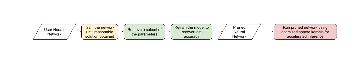
稀疏性背后的总体动机很简单：如果网络中存在零，您可以通过不存储或计算这些参数来优化效率。然而，稀疏性的具体细节很棘手。将参数置为零并不会直接影响模型的延迟/内存开销。

这是因为稠密张量仍然包含被剪枝（零）的元素，而稠密矩阵乘法核仍将对这些元素进行操作。为了实现性能提升，我们需要用稀疏核替换稠密核，稀疏核会跳过涉及被剪枝元素的计算。

为此，这些核在稀疏矩阵上工作，稀疏矩阵不存储被剪枝的元素，而是以压缩格式存储指定的元素。

对于半结构化稀疏性，我们精确地存储一半的原始参数以及一些关于元素如何排列的压缩元数据。

有许多不同的稀疏布局，每种都有其自身的优缺点。2:4 半结构化稀疏布局因两个原因而特别有趣：

• 与以前的稀疏格式不同，半结构化稀疏性旨在在 GPU 上高效加速。2020 年，NVIDIA 通过其 Ampere 架构引入了对半结构化稀疏性的硬件支持，并通过 CUTLASS cuSPARSELt 发布了快速稀疏核。

• 同时，与其它稀疏格式相比，半结构化稀疏性对模型精度的影响往往较小，尤其是在考虑更高级的剪枝/微调方法时。NVIDIA 在其白皮书中表明，一种简单的幅度剪枝范例（一次剪枝到 2:4 稀疏，然后重新训练模型）可以产生几乎相同的模型精度。

半结构化稀疏性处于一个最佳位置，以更低的稀疏度（50%）提供 2 倍（理论上）的加速，同时仍然足够细粒度以保持模型精度。

网络	数据集	指标	稠密 FP16	稀疏 FP16
ResNet-50	ImageNet	Top-1	76.1	76.2
ResNeXt-101_32x8d	ImageNet	Top-1	79.3	79.3
Xception	ImageNet	Top-1	79.2	79.2
SSD-RN50	COCO2017	bbAP	24.8	24.8
MaskRCNN-RN50	COCO2017	bbAP	37.9	37.9
FairSeq Transformer	EN-DE WMT14	BLEU	28.2	28.5
BERT-Large	SQuAD v1.1	F1	91.9	91.9

从工作流角度来看，半结构化稀疏性还具有一个额外的优势。由于稀疏度固定为 50%，因此将模型稀疏化的问题分解为两个不同的子问题变得更容易：

• 准确性 - 我们如何找到一组 2:4 稀疏权重，以最大程度地减少模型准确性下降？

• 性能 - 我们如何加速 2:4 稀疏权重以进行推理并减少内存开销？

\[\begin{bmatrix} 1 & 1 & 0 & 0 \\ 0 & 0 & 1 & 1 \\ 1 & 0 & 0 & 0 \\ 0 & 0 & 1 & 1 \\ \end{bmatrix}\]

这两个问题之间的自然交接点是归零的稠密张量。我们的推理解决方案旨在以这种格式压缩和加速张量。我们预计许多用户会提出自定义掩码解决方案，因为这是一个活跃的研究领域。

现在我们对半结构化稀疏性有了更多了解，让我们将其应用于在问答任务 SQuAD 上训练的 BERT 模型。

介绍与设置

我们首先导入所有需要的包。

# If you are running this in Google Colab, run:
# .. code-block: python
#
#    !pip install datasets transformers evaluate accelerate pandas
#
import os
os.environ["WANDB_DISABLED"] = "true"

import collections
import datasets
import evaluate
import numpy as np
import torch
import torch.utils.benchmark as benchmark
from torch import nn
from torch.sparse import to_sparse_semi_structured, SparseSemiStructuredTensor
from torch.ao.pruning import WeightNormSparsifier
import transformers

# force CUTLASS use if ``cuSPARSELt`` is not available
SparseSemiStructuredTensor._FORCE_CUTLASS = True
torch.manual_seed(100)

# Set default device to "cuda:0"
torch.set_default_device(torch.device("cuda:0" if torch.cuda.is_available() else "cpu"))

我们还需要定义一些特定于数据集/任务的辅助函数。这些函数改编自 此 Hugging Face 课程作为参考。

def preprocess_validation_function(examples, tokenizer):
    inputs = tokenizer(
        [q.strip() for q in examples["question"]],
        examples["context"],
        max_length=384,
        truncation="only_second",
        return_overflowing_tokens=True,
        return_offsets_mapping=True,
        padding="max_length",
    )
    sample_map = inputs.pop("overflow_to_sample_mapping")
    example_ids = []

    for i in range(len(inputs["input_ids"])):
        sample_idx = sample_map[i]
        example_ids.append(examples["id"][sample_idx])
        sequence_ids = inputs.sequence_ids(i)
        offset = inputs["offset_mapping"][i]
        inputs["offset_mapping"][i] = [
            o if sequence_ids[k] == 1 else None for k, o in enumerate(offset)
        ]

    inputs["example_id"] = example_ids
    return inputs


def preprocess_train_function(examples, tokenizer):
    inputs = tokenizer(
        [q.strip() for q in examples["question"]],
        examples["context"],
        max_length=384,
        truncation="only_second",
        return_offsets_mapping=True,
        padding="max_length",
    )

    offset_mapping = inputs["offset_mapping"]
    answers = examples["answers"]
    start_positions = []
    end_positions = []

    for i, (offset, answer) in enumerate(zip(offset_mapping, answers)):
        start_char = answer["answer_start"][0]
        end_char = start_char + len(answer["text"][0])
        sequence_ids = inputs.sequence_ids(i)

        # Find the start and end of the context
        idx = 0
        while sequence_ids[idx] != 1:
            idx += 1
        context_start = idx
        while sequence_ids[idx] == 1:
            idx += 1
        context_end = idx - 1

        # If the answer is not fully inside the context, label it (0, 0)
        if offset[context_start][0] > end_char or offset[context_end][1] < start_char:
            start_positions.append(0)
            end_positions.append(0)
        else:
            # Otherwise it's the start and end token positions
            idx = context_start
            while idx <= context_end and offset[idx][0] <= start_char:
                idx += 1
            start_positions.append(idx - 1)

            idx = context_end
            while idx >= context_start and offset[idx][1] >= end_char:
                idx -= 1
            end_positions.append(idx + 1)

    inputs["start_positions"] = start_positions
    inputs["end_positions"] = end_positions
    return inputs


def compute_metrics(start_logits, end_logits, features, examples):
    n_best = 20
    max_answer_length = 30
    metric = evaluate.load("squad")

    example_to_features = collections.defaultdict(list)
    for idx, feature in enumerate(features):
        example_to_features[feature["example_id"]].append(idx)

    predicted_answers = []
    # for example in ``tqdm`` (examples):
    for example in examples:
        example_id = example["id"]
        context = example["context"]
        answers = []

        # Loop through all features associated with that example
        for feature_index in example_to_features[example_id]:
            start_logit = start_logits[feature_index]
            end_logit = end_logits[feature_index]
            offsets = features[feature_index]["offset_mapping"]

            start_indexes = np.argsort(start_logit)[-1 : -n_best - 1 : -1].tolist()
            end_indexes = np.argsort(end_logit)[-1 : -n_best - 1 : -1].tolist()
            for start_index in start_indexes:
                for end_index in end_indexes:
                    # Skip answers that are not fully in the context
                    if offsets[start_index] is None or offsets[end_index] is None:
                        continue
                    # Skip answers with a length that is either < 0
                    # or > max_answer_length
                    if (
                        end_index < start_index
                        or end_index - start_index + 1 > max_answer_length
                    ):
                        continue

                    answer = {
                        "text": context[
                            offsets[start_index][0] : offsets[end_index][1]
                        ],
                        "logit_score": start_logit[start_index] + end_logit[end_index],
                    }
                    answers.append(answer)

        # Select the answer with the best score
        if len(answers) > 0:
            best_answer = max(answers, key=lambda x: x["logit_score"])
            predicted_answers.append(
                {"id": example_id, "prediction_text": best_answer["text"]}
            )
        else:
            predicted_answers.append({"id": example_id, "prediction_text": ""})

    theoretical_answers = [
        {"id": ex["id"], "answers": ex["answers"]} for ex in examples
    ]
    return metric.compute(predictions=predicted_answers, references=theoretical_answers)

现在这些都已定义，我们只需要一个额外的辅助函数，它将帮助我们对模型进行基准测试。

def measure_execution_time(model, batch_sizes, dataset):
    dataset_for_model = dataset.remove_columns(["example_id", "offset_mapping"])
    dataset_for_model.set_format("torch")
    batch_size_to_time_sec = {}
    for batch_size in batch_sizes:
        batch = {
            k: dataset_for_model[k][:batch_size].cuda()
            for k in dataset_for_model.column_names
        }

        with torch.no_grad():
            baseline_predictions = model(**batch)
            timer = benchmark.Timer(
                stmt="model(**batch)", globals={"model": model, "batch": batch}
            )
            p50 = timer.blocked_autorange().median * 1000
            batch_size_to_time_sec[batch_size] = p50

            model_c = torch.compile(model, fullgraph=True)
            timer = benchmark.Timer(
                stmt="model(**batch)", globals={"model": model_c, "batch": batch}
            )
            p50 = timer.blocked_autorange().median * 1000
            batch_size_to_time_sec[f"{batch_size}_compile"] = p50
            new_predictions = model_c(**batch)

    return batch_size_to_time_sec

我们将首先加载模型和分词器，然后设置我们的数据集。

# load model
model_name = "bert-base-cased"
tokenizer = transformers.AutoTokenizer.from_pretrained(model_name)
model = transformers.AutoModelForQuestionAnswering.from_pretrained(model_name)
print(f"Loading tokenizer: {model_name}")
print(f"Loading model: {model_name}")

# set up train and val dataset
squad_dataset = datasets.load_dataset("squad")
tokenized_squad_dataset = {}
tokenized_squad_dataset["train"] = squad_dataset["train"].map(
    lambda x: preprocess_train_function(x, tokenizer), batched=True
)
tokenized_squad_dataset["validation"] = squad_dataset["validation"].map(
    lambda x: preprocess_validation_function(x, tokenizer),
    batched=True,
    remove_columns=squad_dataset["train"].column_names,
)
data_collator = transformers.DataCollatorWithPadding(tokenizer=tokenizer)

建立基线

接下来，我们将在 SQuAD 上快速训练一个模型的基线。此任务要求我们的模型识别给定上下文（维基百科文章）中回答给定问题的文本跨度或片段。运行以下代码给我一个 F1 分数为 86.9。这与 NVIDIA 报告的分数非常接近，差异可能是由于 BERT-base 与 BERT-large 或微调超参数造成的。

training_args = transformers.TrainingArguments(
    "trainer",
    num_train_epochs=1,
    lr_scheduler_type="constant",
    per_device_train_batch_size=32,
    per_device_eval_batch_size=256,
    logging_steps=50,
    # Limit max steps for tutorial runners. Delete the below line to see the reported accuracy numbers.
    max_steps=500,
    report_to=None,
)

trainer = transformers.Trainer(
    model,
    training_args,
    train_dataset=tokenized_squad_dataset["train"],
    eval_dataset=tokenized_squad_dataset["validation"],
    data_collator=data_collator,
    tokenizer=tokenizer,
)

trainer.train()

# batch sizes to compare for eval
batch_sizes = [4, 16, 64, 256]
# 2:4 sparsity require fp16, so we cast here for a fair comparison
with torch.autocast("cuda"):
    with torch.no_grad():
        predictions = trainer.predict(tokenized_squad_dataset["validation"])
        start_logits, end_logits = predictions.predictions
        fp16_baseline = compute_metrics(
            start_logits,
            end_logits,
            tokenized_squad_dataset["validation"],
            squad_dataset["validation"],
        )
        fp16_time = measure_execution_time(
            model,
            batch_sizes,
            tokenized_squad_dataset["validation"],
        )

print("fp16", fp16_baseline)
print("cuda_fp16 time", fp16_time)

import pandas as pd
df = pd.DataFrame(trainer.state.log_history)
df.plot.line(x='step', y='loss', title="Loss vs. # steps", ylabel="loss")

将 BERT 剪枝为 2:4 稀疏

现在我们有了基线，是时候对 BERT 进行剪枝了。剪枝策略有很多种，但最常见的一种是幅度剪枝，它旨在去除 L1 范数最小的权重。NVIDIA 在其所有结果中都使用了幅度剪枝，它是一个常见的基线。

为此，我们将使用 torch.ao.pruning 包，其中包含一个权重范数（幅度）稀疏器。这些稀疏器通过将掩码参数化应用于模型中的权重张量来工作。这使它们可以通过掩盖剪枝的权重来模拟稀疏性。

我们还必须决定对模型的哪些层应用稀疏性，在这种情况下是所有的 nn.Linear 层，除了特定于任务的头部输出。这是因为半结构化稀疏性有形状约束，而特定于任务的 nn.Linear 层不满足这些约束。

sparsifier = WeightNormSparsifier(
    # apply sparsity to all blocks
    sparsity_level=1.0,
    # shape of 4 elements is a block
    sparse_block_shape=(1, 4),
    # two zeros for every block of 4
    zeros_per_block=2
)

# add to config if ``nn.Linear`` and in the BERT model.
sparse_config = [
    {"tensor_fqn": f"{fqn}.weight"}
    for fqn, module in model.named_modules()
    if isinstance(module, nn.Linear) and "layer" in fqn
]

剪枝模型的第一步是插入用于掩盖模型权重的参数化。这是通过准备步骤完成的。任何时候我们尝试访问 .weight 时，我们都会得到 mask * weight。

# Prepare the model, insert fake-sparsity parametrizations for training
sparsifier.prepare(model, sparse_config)
print(model.bert.encoder.layer[0].output)

然后，我们将执行一次剪枝步骤。所有剪枝器都实现了一个 update_mask() 方法，该方法根据剪枝器实现确定的逻辑更新掩码。步进方法会为稀疏配置中指定的权重调用此 update_mask 函数。

我们还将评估模型，以显示零样本剪枝（即不进行微调/重新训练的剪枝）的精度下降。

sparsifier.step()
with torch.autocast("cuda"):
    with torch.no_grad():
        predictions = trainer.predict(tokenized_squad_dataset["validation"])
    pruned = compute_metrics(
        *predictions.predictions,
        tokenized_squad_dataset["validation"],
        squad_dataset["validation"],
    )
print("pruned eval metrics:", pruned)

在这种状态下，我们可以开始对模型进行微调，更新不会被剪枝的元素，以便更好地弥补精度损失。一旦达到满意状态，我们可以调用 squash_mask 来将掩码和权重融合在一起。这将移除参数化，我们得到一个归零的 2:4 稠密模型。

trainer.train()
sparsifier.squash_mask()
torch.set_printoptions(edgeitems=4)
print(model.bert.encoder.layer[0].intermediate.dense.weight[:8, :8])

df["sparse_loss"] = pd.DataFrame(trainer.state.log_history)["loss"]
df.plot.line(x='step', y=["loss", "sparse_loss"], title="Loss vs. # steps", ylabel="loss")

加速 2:4 稀疏模型进行推理

现在我们拥有这种格式的模型，我们可以像快速入门指南中那样加速它进行推理。

model = model.cuda().half()
# accelerate for sparsity
for fqn, module in model.named_modules():
    if isinstance(module, nn.Linear) and "layer" in fqn:
        module.weight = nn.Parameter(to_sparse_semi_structured(module.weight))

with torch.no_grad():
    predictions = trainer.predict(tokenized_squad_dataset["validation"])
start_logits, end_logits = predictions.predictions
metrics_sparse = compute_metrics(
    start_logits,
    end_logits,
    tokenized_squad_dataset["validation"],
    squad_dataset["validation"],
)
print("sparse eval metrics: ", metrics_sparse)
sparse_perf = measure_execution_time(
    model,
    batch_sizes,
    tokenized_squad_dataset["validation"],
)
print("sparse perf metrics: ", sparse_perf)

在幅度剪枝后重新训练我们的模型，已经恢复了模型剪枝时损失的几乎所有 F1 分数。同时，对于 bs=16，我们实现了 1.28 倍的加速。请注意，并非所有形状都适合性能提升。当批量大小较小且计算稀疏核的时间有限时，它们可能比稠密核慢。

由于半结构化稀疏性被实现为张量子类，因此它与 torch.compile 兼容。当与 to_sparse_semi_structured 结合使用时，我们能够在 BERT 上实现总计 2 倍的加速。

指标	fp16	2:4 稀疏	增量/加速	已编译
精确匹配 (%)	78.53	78.44	-0.09
F1 (%)	86.93	86.49	-0.44
时间 (bs=4)	11.10	15.54	0.71x	否
时间 (bs=16)	19.35	15.74	1.23x	否
时间 (bs=64)	72.71	59.41	1.22x	否
时间 (bs=256)	286.65	247.63	1.14x	否
时间 (bs=4)	7.59	7.46	1.02x	是
时间 (bs=16)	11.47	9.68	1.18x	是
时间 (bs=64)	41.57	36.92	1.13x	是
时间 (bs=256)	159.22	142.23	1.12x	是

结论

在本教程中，我们展示了如何将 BERT 剪枝为 2:4 稀疏，以及如何加速 2:4 稀疏模型进行推理。通过利用我们的 SparseSemiStructuredTensor 子类，我们能够比 fp16 基线实现 1.3 倍的加速，并且在使用 torch.compile 时最高可达 2 倍。我们还通过微调 BERT 来恢复任何损失的 F1 分数（86.92 稠密 vs 86.48 稀疏），从而展示了 2:4 稀疏性的优势。