


注意
跳转到末尾 下载完整的示例代码。
PyTorch 神经风格迁移#
创建于:2017年4月6日 | 最后更新:2024年1月19日 | 最后验证:2024年11月5日
作者: Alexis Jacq
编辑: Winston Herring
简介#
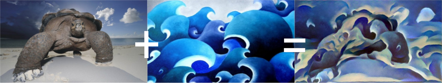
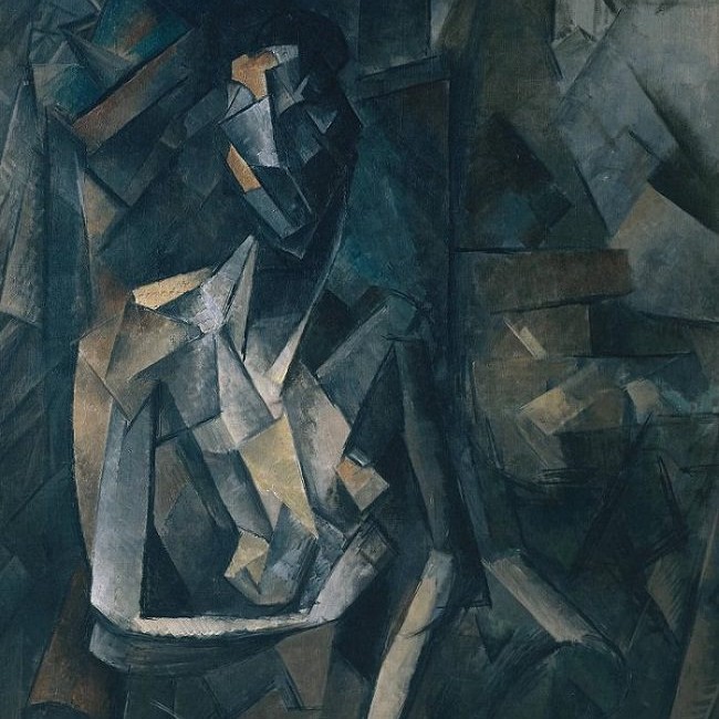
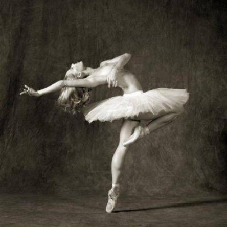
本教程将解释如何实现由 Leon A. Gatys、Alexander S. Ecker 和 Matthias Bethge 开发的 Neural-Style 算法。Neural-Style,也称为 Neural-Transfer,允许您将一张图片以新的艺术风格进行重现。该算法需要三张图片:一张输入图片、一张内容图片和一张风格图片,然后修改输入图片,使其在内容上类似于内容图片,在艺术风格上类似于风格图片。
基本原理#
原理很简单:我们定义两种距离,一种是内容距离(\(D_C\)),另一种是风格距离(\(D_S\))。\(D_C\) 衡量两张图片在内容上的差异,而 \(D_S\) 衡量两张图片在风格上的差异。然后,我们取第三张图片,即输入图片,并对其进行转换,以最小化它与内容图片的**内容距离**以及它与风格图片的**风格距离**。现在我们可以导入必要的包,并开始神经风格迁移。
导入包和选择设备#
以下是实现神经风格迁移所需的包列表。
torch,torch.nn,numpy(使用 PyTorch 进行神经网络的必备包)torch.optim(高效的梯度下降)PIL,PIL.Image,matplotlib.pyplot(加载和显示图片)torchvision.transforms(将 PIL 图片转换为张量)torchvision.models(训练或加载预训练模型)copy(用于深度复制模型;系统包)
import torch
import torch.nn as nn
import torch.nn.functional as F
import torch.optim as optim

from PIL import Image
import matplotlib.pyplot as plt

import torchvision.transforms as transforms
from torchvision.models import vgg19, VGG19_Weights

import copy
接下来,我们需要选择在哪个设备上运行网络,并导入内容图片和风格图片。对大型图片进行神经风格迁移算法的计算耗时较长,在 GPU 上运行会快得多。我们可以使用 torch.cuda.is_available() 来检测是否可用 GPU。然后,我们设置 torch.device 以供整个教程使用。此外,.to(device) 方法用于将张量或模块移动到目标设备。
device = torch.device("cuda" if torch.cuda.is_available() else "cpu")
torch.set_default_device(device)
加载图片#
现在我们将导入风格图片和内容图片。原始的 PIL 图片的像素值在 0 到 255 之间,但转换为 torch 张量后,其值会被转换为 0 到 1 之间。图片还需要调整大小以具有相同的尺寸。需要注意的一个重要细节是,PyTorch 库中的神经网络是以像素值在 0 到 1 之间的张量进行训练的。如果您尝试将 0 到 255 的张量图片输入网络,那么激活的特征图将无法感知预期的内容和风格。然而,Caffe 库中的预训练网络是以 0 到 255 的张量图片进行训练的。
注意
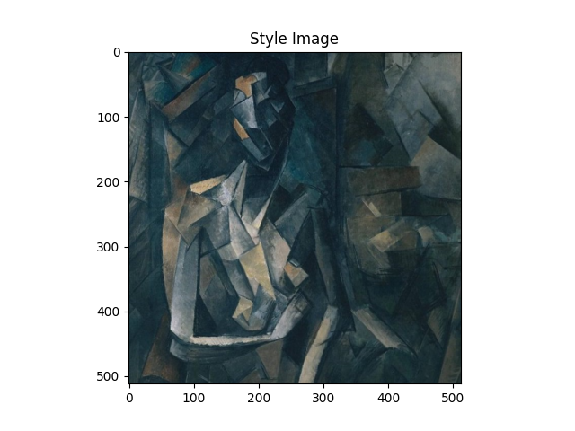
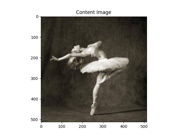
以下是运行本教程所需的图片下载链接:picasso.jpg 和 dancing.jpg。下载这两张图片,并将它们添加到当前工作目录下的一个名为 images 的文件夹中。
# desired size of the output image
imsize = 512 if torch.cuda.is_available() else 128  # use small size if no GPU

loader = transforms.Compose([
    transforms.Resize(imsize),  # scale imported image
    transforms.ToTensor()])  # transform it into a torch tensor


def image_loader(image_name):
    image = Image.open(image_name)
    # fake batch dimension required to fit network's input dimensions
    image = loader(image).unsqueeze(0)
    return image.to(device, torch.float)


style_img = image_loader("./data/images/neural-style/picasso.jpg")
content_img = image_loader("./data/images/neural-style/dancing.jpg")

assert style_img.size() == content_img.size(), \
    "we need to import style and content images of the same size"
现在,让我们创建一个函数来显示图片,通过将图片的副本转换回 PIL 格式,并使用 plt.imshow 显示该副本。我们将尝试显示内容图片和风格图片,以确保它们已正确导入。
unloader = transforms.ToPILImage()  # reconvert into PIL image

plt.ion()

def imshow(tensor, title=None):
    image = tensor.cpu().clone()  # we clone the tensor to not do changes on it
    image = image.squeeze(0)      # remove the fake batch dimension
    image = unloader(image)
    plt.imshow(image)
    if title is not None:
        plt.title(title)
    plt.pause(0.001) # pause a bit so that plots are updated


plt.figure()
imshow(style_img, title='Style Image')

plt.figure()
imshow(content_img, title='Content Image')
损失函数#
内容损失#
内容损失函数表示单个层的内容距离的加权版本。该函数接收处理输入 \(X\) 的网络中层 \(L\) 的特征图 \(F_{XL}\),并返回图片 \(X\) 和内容图片 \(C\) 之间的加权内容距离 \(w_{CL}.D_C^L(X,C)\)。为了计算内容距离,函数必须能够访问内容图片的特征图(\(F_{CL}\))。我们将其实现为一个 PyTorch 模块,其构造函数接收 \(F_{CL}\) 作为输入。距离 \(\|F_{XL} - F_{CL}\|^2\) 是两个特征图集之间的均方误差,可以使用 nn.MSELoss 计算。
我们将此内容损失模块直接添加到用于计算内容距离的卷积层之后。这样,每次网络接收输入图片时,内容损失将在所需层计算,并且由于自动求导,所有梯度都将被计算。现在,为了使内容损失层透明,我们必须定义一个 forward 方法,该方法计算内容损失,然后返回层的输入。计算出的损失将作为模块的参数保存。
class ContentLoss(nn.Module):

    def __init__(self, target,):
        super(ContentLoss, self).__init__()
        # we 'detach' the target content from the tree used
        # to dynamically compute the gradient: this is a stated value,
        # not a variable. Otherwise the forward method of the criterion
        # will throw an error.
        self.target = target.detach()

    def forward(self, input):
        self.loss = F.mse_loss(input, self.target)
        return input
注意
重要细节:尽管此模块名为 ContentLoss,但它不是真正的 PyTorch 损失函数。如果您想将内容损失定义为 PyTorch 损失函数,则必须创建一个 PyTorch 自动求导函数,在 backward 方法中手动重新计算/实现梯度。
风格损失#
风格损失模块的实现方式与内容损失模块非常相似。它将充当网络中计算该层风格损失的透明层。为了计算风格损失,我们需要计算 Gram 矩阵 \(G_{XL}\)。Gram 矩阵是将给定矩阵与其转置矩阵相乘的结果。在此应用中,给定矩阵是层 \(L\) 的特征图 \(F_{XL}\) 的重塑版本。\(F_{XL}\) 被重塑为 \(\hat{F}_{XL}\),一个 \(K\) x \(N\) 的矩阵,其中 \(K\) 是层 \(L\) 处的特征图数量,\(N\) 是任何矢量化特征图 \(F_{XL}^k\) 的长度。例如,\(\hat{F}_{XL}\) 的第一行对应于第一个矢量化特征图 \(F_{XL}^1\)。
最后,必须通过将 Gram 矩阵的每个元素除以矩阵中元素的总数来对其进行归一化。此归一化是为了抵消 \(\hat{F}_{XL}\) 矩阵具有较大的 \(N\) 维度会导致 Gram 矩阵中值较大的事实。这些较大的值将导致网络的前几层(池化层之前)在梯度下降过程中产生更大的影响。风格特征往往存在于网络的更深层,因此此归一化步骤至关重要。
def gram_matrix(input):
    a, b, c, d = input.size()  # a=batch size(=1)
    # b=number of feature maps
    # (c,d)=dimensions of a f. map (N=c*d)

    features = input.view(a * b, c * d)  # resize F_XL into \hat F_XL

    G = torch.mm(features, features.t())  # compute the gram product

    # we 'normalize' the values of the gram matrix
    # by dividing by the number of element in each feature maps.
    return G.div(a * b * c * d)
现在,风格损失模块与内容损失模块几乎完全相同。风格距离也是通过 \(G_{XL}\) 和 \(G_{SL}\) 之间的均方误差来计算的。
class StyleLoss(nn.Module):

    def __init__(self, target_feature):
        super(StyleLoss, self).__init__()
        self.target = gram_matrix(target_feature).detach()

    def forward(self, input):
        G = gram_matrix(input)
        self.loss = F.mse_loss(G, self.target)
        return input
导入模型#
现在我们需要导入一个预训练的神经网络。我们将使用论文中使用的 19 层 VGG 网络。
PyTorch 对 VGG 的实现是一个模块,分为两个子 Sequential 模块:features(包含卷积层和池化层)和 classifier(包含全连接层)。我们将使用 features 模块,因为我们需要单独的卷积层的输出来衡量内容和风格损失。某些层在训练和评估期间的行为不同,因此我们必须使用 .eval() 将网络设置为评估模式。
cnn = vgg19(weights=VGG19_Weights.DEFAULT).features.eval()
Downloading: "https://download.pytorch.org/models/vgg19-dcbb9e9d.pth" to /var/lib/ci-user/.cache/torch/hub/checkpoints/vgg19-dcbb9e9d.pth

  0%|          | 0.00/548M [00:00<?, ?B/s]
  5%|▌         | 29.6M/548M [00:00<00:01, 310MB/s]
 11%|█         | 60.9M/548M [00:00<00:01, 320MB/s]
 17%|█▋        | 92.1M/548M [00:00<00:01, 323MB/s]
 23%|██▎       | 123M/548M [00:00<00:01, 325MB/s]
 28%|██▊       | 155M/548M [00:00<00:01, 325MB/s]
 34%|███▍      | 186M/548M [00:00<00:01, 325MB/s]
 40%|███▉      | 217M/548M [00:00<00:01, 326MB/s]
 45%|████▌     | 248M/548M [00:00<00:00, 326MB/s]
 51%|█████     | 280M/548M [00:00<00:00, 327MB/s]
 57%|█████▋    | 311M/548M [00:01<00:00, 327MB/s]
 62%|██████▏   | 342M/548M [00:01<00:00, 327MB/s]
 68%|██████▊   | 374M/548M [00:01<00:00, 328MB/s]
 74%|███████▍  | 405M/548M [00:01<00:00, 328MB/s]
 80%|███████▉  | 436M/548M [00:01<00:00, 328MB/s]
 85%|████████▌ | 467M/548M [00:01<00:00, 327MB/s]
 91%|█████████ | 499M/548M [00:01<00:00, 327MB/s]
 97%|█████████▋| 530M/548M [00:01<00:00, 327MB/s]
100%|██████████| 548M/548M [00:01<00:00, 327MB/s]
此外,VGG 网络使用均值为 [0.485, 0.456, 0.406]、标准差为 [0.229, 0.224, 0.225] 的通道进行图像归一化。在将图像输入网络之前,我们将使用这些值对其进行归一化。
cnn_normalization_mean = torch.tensor([0.485, 0.456, 0.406])
cnn_normalization_std = torch.tensor([0.229, 0.224, 0.225])

# create a module to normalize input image so we can easily put it in a
# ``nn.Sequential``
class Normalization(nn.Module):
    def __init__(self, mean, std):
        super(Normalization, self).__init__()
        # .view the mean and std to make them [C x 1 x 1] so that they can
        # directly work with image Tensor of shape [B x C x H x W].
        # B is batch size. C is number of channels. H is height and W is width.
        self.mean = torch.tensor(mean).view(-1, 1, 1)
        self.std = torch.tensor(std).view(-1, 1, 1)

    def forward(self, img):
        # normalize ``img``
        return (img - self.mean) / self.std
一个 Sequential 模块包含一个子模块的有序列表。例如,vgg19.features 包含一个按深度顺序排列的序列(Conv2d、ReLU、MaxPool2d、Conv2d、ReLU…)。我们需要将内容损失和风格损失层插入到它们所检测的卷积层之后。为此,我们必须创建一个新的 Sequential 模块,其中正确地插入了内容损失和风格损失模块。
# desired depth layers to compute style/content losses :
content_layers_default = ['conv_4']
style_layers_default = ['conv_1', 'conv_2', 'conv_3', 'conv_4', 'conv_5']

def get_style_model_and_losses(cnn, normalization_mean, normalization_std,
                               style_img, content_img,
                               content_layers=content_layers_default,
                               style_layers=style_layers_default):
    # normalization module
    normalization = Normalization(normalization_mean, normalization_std)

    # just in order to have an iterable access to or list of content/style
    # losses
    content_losses = []
    style_losses = []

    # assuming that ``cnn`` is a ``nn.Sequential``, so we make a new ``nn.Sequential``
    # to put in modules that are supposed to be activated sequentially
    model = nn.Sequential(normalization)

    i = 0  # increment every time we see a conv
    for layer in cnn.children():
        if isinstance(layer, nn.Conv2d):
            i += 1
            name = 'conv_{}'.format(i)
        elif isinstance(layer, nn.ReLU):
            name = 'relu_{}'.format(i)
            # The in-place version doesn't play very nicely with the ``ContentLoss``
            # and ``StyleLoss`` we insert below. So we replace with out-of-place
            # ones here.
            layer = nn.ReLU(inplace=False)
        elif isinstance(layer, nn.MaxPool2d):
            name = 'pool_{}'.format(i)
        elif isinstance(layer, nn.BatchNorm2d):
            name = 'bn_{}'.format(i)
        else:
            raise RuntimeError('Unrecognized layer: {}'.format(layer.__class__.__name__))

        model.add_module(name, layer)

        if name in content_layers:
            # add content loss:
            target = model(content_img).detach()
            content_loss = ContentLoss(target)
            model.add_module("content_loss_{}".format(i), content_loss)
            content_losses.append(content_loss)

        if name in style_layers:
            # add style loss:
            target_feature = model(style_img).detach()
            style_loss = StyleLoss(target_feature)
            model.add_module("style_loss_{}".format(i), style_loss)
            style_losses.append(style_loss)

    # now we trim off the layers after the last content and style losses
    for i in range(len(model) - 1, -1, -1):
        if isinstance(model[i], ContentLoss) or isinstance(model[i], StyleLoss):
            break

    model = model[:(i + 1)]

    return model, style_losses, content_losses
接下来,我们选择输入图片。您可以使用内容图片的副本或白噪声。
input_img = content_img.clone()
# if you want to use white noise by using the following code:
#
# .. code-block:: python
#
#    input_img = torch.randn(content_img.data.size())

# add the original input image to the figure:
plt.figure()
imshow(input_img, title='Input Image')

梯度下降#
正如算法的作者 Leon Gatys 在 这里 建议的那样,我们将使用 L-BFGS 算法进行梯度下降。与训练网络不同,我们希望通过训练输入图片来最小化内容/风格损失。我们将创建一个 PyTorch L-BFGS 优化器 optim.LBFGS,并将图片作为要优化的张量传递给它。
def get_input_optimizer(input_img):
    # this line to show that input is a parameter that requires a gradient
    optimizer = optim.LBFGS([input_img])
    return optimizer
最后,我们必须定义一个执行神经风格迁移的函数。对于网络的每一次迭代,它都会接收更新后的输入并计算新的损失。我们将调用每个损失模块的 backward 方法来动态计算它们的梯度。优化器需要一个“closure”函数,该函数会重新评估模块并返回损失。
我们还有一个最终约束需要解决。网络可能会尝试使用超出图片 0 到 1 张量范围的值来优化输入。我们可以通过每次运行网络时将输入值修正到 0 到 1 之间来解决这个问题。
def run_style_transfer(cnn, normalization_mean, normalization_std,
                       content_img, style_img, input_img, num_steps=300,
                       style_weight=1000000, content_weight=1):
    """Run the style transfer."""
    print('Building the style transfer model..')
    model, style_losses, content_losses = get_style_model_and_losses(cnn,
        normalization_mean, normalization_std, style_img, content_img)

    # We want to optimize the input and not the model parameters so we
    # update all the requires_grad fields accordingly
    input_img.requires_grad_(True)
    # We also put the model in evaluation mode, so that specific layers
    # such as dropout or batch normalization layers behave correctly.
    model.eval()
    model.requires_grad_(False)

    optimizer = get_input_optimizer(input_img)

    print('Optimizing..')
    run = [0]
    while run[0] <= num_steps:

        def closure():
            # correct the values of updated input image
            with torch.no_grad():
                input_img.clamp_(0, 1)

            optimizer.zero_grad()
            model(input_img)
            style_score = 0
            content_score = 0

            for sl in style_losses:
                style_score += sl.loss
            for cl in content_losses:
                content_score += cl.loss

            style_score *= style_weight
            content_score *= content_weight

            loss = style_score + content_score
            loss.backward()

            run[0] += 1
            if run[0] % 50 == 0:
                print("run {}:".format(run))
                print('Style Loss : {:4f} Content Loss: {:4f}'.format(
                    style_score.item(), content_score.item()))
                print()

            return style_score + content_score

        optimizer.step(closure)

    # a last correction...
    with torch.no_grad():
        input_img.clamp_(0, 1)

    return input_img
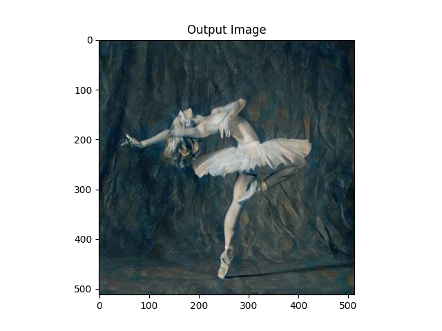
最后,我们可以运行该算法。
output = run_style_transfer(cnn, cnn_normalization_mean, cnn_normalization_std,
                            content_img, style_img, input_img)

plt.figure()
imshow(output, title='Output Image')

# sphinx_gallery_thumbnail_number = 4
plt.ioff()
plt.show()
Building the style transfer model..
/usr/local/lib/python3.10/dist-packages/torch/utils/_device.py:103: UserWarning:

To copy construct from a tensor, it is recommended to use sourceTensor.detach().clone() or sourceTensor.detach().clone().requires_grad_(True), rather than torch.tensor(sourceTensor).

Optimizing..
run [50]:
Style Loss : 4.048831 Content Loss: 4.154776

run [100]:
Style Loss : 1.127818 Content Loss: 3.011050

run [150]:
Style Loss : 0.706650 Content Loss: 2.643324

run [200]:
Style Loss : 0.474288 Content Loss: 2.487212

run [250]:
Style Loss : 0.341487 Content Loss: 2.397301

run [300]:
Style Loss : 0.261463 Content Loss: 2.345904
脚本总运行时间: (0 分钟 12.654 秒)
