beginner/knowledge_distillation_tutorial

在 Google Colab 中运行

Colab

下载 Notebook

Notebook

在 GitHub 上查看

GitHub

知识蒸馏教程

创建日期：2023 年 8 月 22 日 | 最后更新：2025 年 1 月 24 日 | 最后验证：2024 年 11 月 5 日

作者: Alexandros Chariton

知识蒸馏是一种技术，可以将在计算上昂贵的大型模型中的知识转移到较小的模型中，而不会失去有效性。这使得模型可以在性能较低的硬件上部署，从而使评估更快、更高效。

在本教程中，我们将进行一系列实验，重点是提高轻量级神经网络的准确性，使用更强大的网络作为教师。轻量级网络的计算成本和速度将保持不变，我们的干预只关注其权重，而不关注其前向传播。这项技术的应用可以在无人机或手机等设备中找到。在本教程中，我们不使用任何外部包，因为我们所需的一切都可以在 torch 和 torchvision 中获得。

在本教程中，您将学习

• 如何修改模型类以提取隐藏表示并将其用于进一步计算

• 如何修改 PyTorch 中的常规训练循环以在例如分类交叉熵之外包含额外的损失

• 如何通过使用更复杂的模型作为教师来提高轻量级模型的性能

先决条件

• 1 个 GPU，4GB 内存

• PyTorch v2.0 或更高版本

• CIFAR-10 数据集（由脚本下载并保存到名为 /data 的目录中）

import torch
import torch.nn as nn
import torch.optim as optim
import torchvision.transforms as transforms
import torchvision.datasets as datasets

# Check if the current `accelerator <https://pytorch.ac.cn/docs/stable/torch.html#accelerators>`__
# is available, and if not, use the CPU
device = torch.accelerator.current_accelerator().type if torch.accelerator.is_available() else "cpu"
print(f"Using {device} device")

Using cuda device

加载 CIFAR-10

CIFAR-10 是一个流行的图像数据集，包含十个类别。我们的目标是为每个输入图像预测以下类别之一。

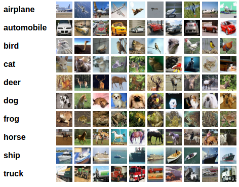
CIFAR-10 图像示例

输入图像是 RGB 格式，因此它们有 3 个通道，大小为 32x32 像素。基本上，每个图像由 3 x 32 x 32 = 3072 个介于 0 到 255 之间的数字描述。神经网络中的常见做法是标准化输入，这样做有多种原因，包括避免常用激活函数的饱和并提高数值稳定性。我们的标准化过程包括减去均值并除以每个通道的标准差。张量“mean=[0.485, 0.456, 0.406]”和“std=[0.229, 0.224, 0.225]”已经计算出来，它们表示 CIFAR-10 预定义训练集子集中每个通道的均值和标准差。请注意，我们也将这些值用于测试集，而无需从头重新计算均值和标准差。这是因为网络是根据上述数字减去和除以产生的特征进行训练的，我们希望保持一致性。此外，在现实生活中，我们将无法计算测试集的均值和标准差，因为在我们的假设下，这些数据在那个时候是无法访问的。

最后一点，我们通常将这个保留集称为验证集，并且在优化模型在验证集上的性能后，我们使用一个单独的集合，称为测试集。这样做是为了避免基于单一指标的贪婪和有偏优化来选择模型。

# Below we are preprocessing data for CIFAR-10. We use an arbitrary batch size of 128.
transforms_cifar = transforms.Compose([
    transforms.ToTensor(),
    transforms.Normalize(mean=[0.485, 0.456, 0.406], std=[0.229, 0.224, 0.225]),
])

# Loading the CIFAR-10 dataset:
train_dataset = datasets.CIFAR10(root='./data', train=True, download=True, transform=transforms_cifar)
test_dataset = datasets.CIFAR10(root='./data', train=False, download=True, transform=transforms_cifar)

  0%|          | 0.00/170M [00:00<?, ?B/s]
  0%|          | 459k/170M [00:00<00:37, 4.57MB/s]
  5%|▍         | 8.03M/170M [00:00<00:03, 46.3MB/s]
 11%|█▏        | 19.4M/170M [00:00<00:01, 77.2MB/s]
 18%|█▊        | 30.7M/170M [00:00<00:01, 91.2MB/s]
 25%|██▍       | 42.1M/170M [00:00<00:01, 99.4MB/s]
 31%|███▏      | 53.5M/170M [00:00<00:01, 104MB/s]
 38%|███▊      | 65.0M/170M [00:00<00:00, 108MB/s]
 45%|████▍     | 76.3M/170M [00:00<00:00, 109MB/s]
 51%|█████▏    | 87.6M/170M [00:00<00:00, 111MB/s]
 58%|█████▊    | 98.9M/170M [00:01<00:00, 111MB/s]
 65%|██████▍   | 110M/170M [00:01<00:00, 112MB/s]
 71%|███████▏  | 122M/170M [00:01<00:00, 112MB/s]
 78%|███████▊  | 133M/170M [00:01<00:00, 113MB/s]
 85%|████████▍ | 144M/170M [00:01<00:00, 113MB/s]
 91%|█████████▏| 156M/170M [00:01<00:00, 113MB/s]
 98%|█████████▊| 167M/170M [00:01<00:00, 113MB/s]
100%|██████████| 170M/170M [00:01<00:00, 104MB/s]

注意

本节仅适用于对快速结果感兴趣的 CPU 用户。仅当您对小规模实验感兴趣时才使用此选项。请记住，使用任何 GPU 运行代码都应该相当快。仅从训练/测试数据集中选择前 num_images_to_keep 个图像

#from torch.utils.data import Subset
#num_images_to_keep = 2000
#train_dataset = Subset(train_dataset, range(min(num_images_to_keep, 50_000)))
#test_dataset = Subset(test_dataset, range(min(num_images_to_keep, 10_000)))

#Dataloaders
train_loader = torch.utils.data.DataLoader(train_dataset, batch_size=128, shuffle=True, num_workers=2)
test_loader = torch.utils.data.DataLoader(test_dataset, batch_size=128, shuffle=False, num_workers=2)

定义模型类和实用函数

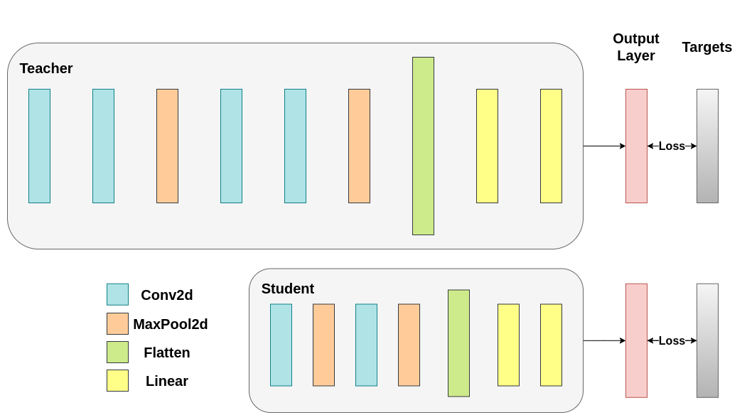
接下来，我们需要定义模型类。这里需要设置几个用户定义的参数。我们使用两种不同的架构，在我们的实验中保持滤波器数量固定以确保公平比较。两种架构都是卷积神经网络（CNN），具有不同数量的卷积层作为特征提取器，然后是具有 10 个类别的分类器。学生的滤波器和神经元数量较少。

# Deeper neural network class to be used as teacher:
class DeepNN(nn.Module):
    def __init__(self, num_classes=10):
        super(DeepNN, self).__init__()
        self.features = nn.Sequential(
            nn.Conv2d(3, 128, kernel_size=3, padding=1),
            nn.ReLU(),
            nn.Conv2d(128, 64, kernel_size=3, padding=1),
            nn.ReLU(),
            nn.MaxPool2d(kernel_size=2, stride=2),
            nn.Conv2d(64, 64, kernel_size=3, padding=1),
            nn.ReLU(),
            nn.Conv2d(64, 32, kernel_size=3, padding=1),
            nn.ReLU(),
            nn.MaxPool2d(kernel_size=2, stride=2),
        )
        self.classifier = nn.Sequential(
            nn.Linear(2048, 512),
            nn.ReLU(),
            nn.Dropout(0.1),
            nn.Linear(512, num_classes)
        )

    def forward(self, x):
        x = self.features(x)
        x = torch.flatten(x, 1)
        x = self.classifier(x)
        return x

# Lightweight neural network class to be used as student:
class LightNN(nn.Module):
    def __init__(self, num_classes=10):
        super(LightNN, self).__init__()
        self.features = nn.Sequential(
            nn.Conv2d(3, 16, kernel_size=3, padding=1),
            nn.ReLU(),
            nn.MaxPool2d(kernel_size=2, stride=2),
            nn.Conv2d(16, 16, kernel_size=3, padding=1),
            nn.ReLU(),
            nn.MaxPool2d(kernel_size=2, stride=2),
        )
        self.classifier = nn.Sequential(
            nn.Linear(1024, 256),
            nn.ReLU(),
            nn.Dropout(0.1),
            nn.Linear(256, num_classes)
        )

    def forward(self, x):
        x = self.features(x)
        x = torch.flatten(x, 1)
        x = self.classifier(x)
        return x

我们使用 2 个函数来帮助我们生成和评估原始分类任务的结果。其中一个函数名为 train，它接受以下参数：

• model: 通过此函数训练（更新其权重）的模型实例。

• train_loader: 我们在上面定义了 train_loader，它的作用是将数据馈送到模型中。

• epochs: 我们循环数据集的次数。

• learning_rate: 学习率决定了我们向收敛迈进的步长。步长过大或过小都可能有害。

• device: 确定运行工作负载的设备。可以是 CPU 或 GPU，具体取决于可用性。

我们的测试函数类似，但它将使用 test_loader 调用，以从测试集中加载图像。

使用交叉熵训练两个网络。学生将用作基线：

def train(model, train_loader, epochs, learning_rate, device):
    criterion = nn.CrossEntropyLoss()
    optimizer = optim.Adam(model.parameters(), lr=learning_rate)

    model.train()

    for epoch in range(epochs):
        running_loss = 0.0
        for inputs, labels in train_loader:
            # inputs: A collection of batch_size images
            # labels: A vector of dimensionality batch_size with integers denoting class of each image
            inputs, labels = inputs.to(device), labels.to(device)

            optimizer.zero_grad()
            outputs = model(inputs)

            # outputs: Output of the network for the collection of images. A tensor of dimensionality batch_size x num_classes
            # labels: The actual labels of the images. Vector of dimensionality batch_size
            loss = criterion(outputs, labels)
            loss.backward()
            optimizer.step()

            running_loss += loss.item()

        print(f"Epoch {epoch+1}/{epochs}, Loss: {running_loss / len(train_loader)}")

def test(model, test_loader, device):
    model.to(device)
    model.eval()

    correct = 0
    total = 0

    with torch.no_grad():
        for inputs, labels in test_loader:
            inputs, labels = inputs.to(device), labels.to(device)

            outputs = model(inputs)
            _, predicted = torch.max(outputs.data, 1)

            total += labels.size(0)
            correct += (predicted == labels).sum().item()

    accuracy = 100 * correct / total
    print(f"Test Accuracy: {accuracy:.2f}%")
    return accuracy

交叉熵运行

为了可重现性，我们需要设置 torch 手动种子。我们使用不同的方法训练网络，因此为了公平比较，用相同的权重初始化网络是有意义的。首先使用交叉熵训练教师网络

torch.manual_seed(42)
nn_deep = DeepNN(num_classes=10).to(device)
train(nn_deep, train_loader, epochs=10, learning_rate=0.001, device=device)
test_accuracy_deep = test(nn_deep, test_loader, device)

# Instantiate the lightweight network:
torch.manual_seed(42)
nn_light = LightNN(num_classes=10).to(device)

Epoch 1/10, Loss: 1.3391602060678975
Epoch 2/10, Loss: 0.8713056307924373
Epoch 3/10, Loss: 0.6801400981138429
Epoch 4/10, Loss: 0.5297792153742612
Epoch 5/10, Loss: 0.40570281122041785
Epoch 6/10, Loss: 0.30292498615696606
Epoch 7/10, Loss: 0.2076736916514004
Epoch 8/10, Loss: 0.15907087967828717
Epoch 9/10, Loss: 0.13937283643638082
Epoch 10/10, Loss: 0.11684243535846853
Test Accuracy: 74.58%

我们再实例化一个轻量级网络模型来比较它们的性能。反向传播对权重初始化很敏感，因此我们需要确保这两个网络具有完全相同的初始化。

torch.manual_seed(42)
new_nn_light = LightNN(num_classes=10).to(device)

为了确保我们已经创建了第一个网络的副本，我们检查其第一层的范数。如果匹配，那么我们可以安全地得出结论，这些网络确实是相同的。

# Print the norm of the first layer of the initial lightweight model
print("Norm of 1st layer of nn_light:", torch.norm(nn_light.features[0].weight).item())
# Print the norm of the first layer of the new lightweight model
print("Norm of 1st layer of new_nn_light:", torch.norm(new_nn_light.features[0].weight).item())

Norm of 1st layer of nn_light: 2.327361822128296
Norm of 1st layer of new_nn_light: 2.327361822128296

打印每个模型中的总参数数量

total_params_deep = "{:,}".format(sum(p.numel() for p in nn_deep.parameters()))
print(f"DeepNN parameters: {total_params_deep}")
total_params_light = "{:,}".format(sum(p.numel() for p in nn_light.parameters()))
print(f"LightNN parameters: {total_params_light}")

DeepNN parameters: 1,186,986
LightNN parameters: 267,738

使用交叉熵损失训练和测试轻量级网络

train(nn_light, train_loader, epochs=10, learning_rate=0.001, device=device)
test_accuracy_light_ce = test(nn_light, test_loader, device)

Epoch 1/10, Loss: 1.466814213396643
Epoch 2/10, Loss: 1.1520665068455669
Epoch 3/10, Loss: 1.0208662809313411
Epoch 4/10, Loss: 0.9202409523832219
Epoch 5/10, Loss: 0.8444143893468715
Epoch 6/10, Loss: 0.7782444348725517
Epoch 7/10, Loss: 0.7122745978862733
Epoch 8/10, Loss: 0.6551048502592784
Epoch 9/10, Loss: 0.5984768202847532
Epoch 10/10, Loss: 0.5492785314617254
Test Accuracy: 70.03%

正如我们所看到的，根据测试准确性，我们现在可以将用作教师的更深层网络与我们所谓的学生轻量级网络进行比较。到目前为止，我们的学生还没有干预教师，因此这个性能是学生自己实现的。到目前为止的指标可以通过以下几行代码查看

print(f"Teacher accuracy: {test_accuracy_deep:.2f}%")
print(f"Student accuracy: {test_accuracy_light_ce:.2f}%")

Teacher accuracy: 74.58%
Student accuracy: 70.03%

知识蒸馏运行

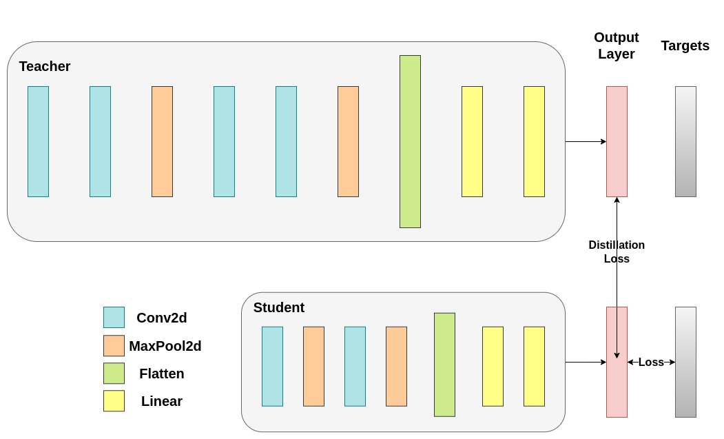
现在让我们尝试通过整合教师来提高学生网络的测试准确率。知识蒸馏是一种直接实现此目标的技术，它基于这样一个事实：两个网络都输出关于我们类别的概率分布。因此，两个网络共享相同数量的输出神经元。该方法的工作原理是在传统的交叉熵损失中加入一个额外的损失，该损失基于教师网络的 softmax 输出。假设经过适当训练的教师网络的输出激活携带了额外的、可供学生网络在训练期间利用的信息。原始工作表明，利用软目标中较小概率的比率有助于实现深度神经网络的潜在目标，即在数据上创建相似性结构，使相似的物体更靠近地映射。例如，在 CIFAR-10 中，如果存在车轮，卡车可能会被误认为是汽车或飞机，但不太可能被误认为是狗。因此，假设有价值的信息不仅存在于经过适当训练的模型的前向预测中，而且存在于整个输出分布中是合乎情理的。然而，单独的交叉熵不足以利用这些信息，因为非预测类别的激活往往太小，导致传播的梯度无法有意义地改变权重以构建这种理想的向量空间。

当我们继续定义第一个引入师生动态的辅助函数时，我们需要包含一些额外的参数

• T: 温度控制输出分布的平滑度。较大的 T 导致更平滑的分布，从而使较小的概率获得更大的提升。

• soft_target_loss_weight: 分配给我们即将包含的额外目标的一个权重。

• ce_loss_weight: 分配给交叉熵的权重。调整这些权重会促使网络向优化任一目标的方向发展。

蒸馏损失从网络的 logits 计算。它只向学生返回梯度：

def train_knowledge_distillation(teacher, student, train_loader, epochs, learning_rate, T, soft_target_loss_weight, ce_loss_weight, device):
    ce_loss = nn.CrossEntropyLoss()
    optimizer = optim.Adam(student.parameters(), lr=learning_rate)

    teacher.eval()  # Teacher set to evaluation mode
    student.train() # Student to train mode

    for epoch in range(epochs):
        running_loss = 0.0
        for inputs, labels in train_loader:
            inputs, labels = inputs.to(device), labels.to(device)

            optimizer.zero_grad()

            # Forward pass with the teacher model - do not save gradients here as we do not change the teacher's weights
            with torch.no_grad():
                teacher_logits = teacher(inputs)

            # Forward pass with the student model
            student_logits = student(inputs)

            #Soften the student logits by applying softmax first and log() second
            soft_targets = nn.functional.softmax(teacher_logits / T, dim=-1)
            soft_prob = nn.functional.log_softmax(student_logits / T, dim=-1)

            # Calculate the soft targets loss. Scaled by T**2 as suggested by the authors of the paper "Distilling the knowledge in a neural network"
            soft_targets_loss = torch.sum(soft_targets * (soft_targets.log() - soft_prob)) / soft_prob.size()[0] * (T**2)

            # Calculate the true label loss
            label_loss = ce_loss(student_logits, labels)

            # Weighted sum of the two losses
            loss = soft_target_loss_weight * soft_targets_loss + ce_loss_weight * label_loss

            loss.backward()
            optimizer.step()

            running_loss += loss.item()

        print(f"Epoch {epoch+1}/{epochs}, Loss: {running_loss / len(train_loader)}")

# Apply ``train_knowledge_distillation`` with a temperature of 2. Arbitrarily set the weights to 0.75 for CE and 0.25 for distillation loss.
train_knowledge_distillation(teacher=nn_deep, student=new_nn_light, train_loader=train_loader, epochs=10, learning_rate=0.001, T=2, soft_target_loss_weight=0.25, ce_loss_weight=0.75, device=device)
test_accuracy_light_ce_and_kd = test(new_nn_light, test_loader, device)

# Compare the student test accuracy with and without the teacher, after distillation
print(f"Teacher accuracy: {test_accuracy_deep:.2f}%")
print(f"Student accuracy without teacher: {test_accuracy_light_ce:.2f}%")
print(f"Student accuracy with CE + KD: {test_accuracy_light_ce_and_kd:.2f}%")

Epoch 1/10, Loss: 2.406861845794541
Epoch 2/10, Loss: 1.8864121251094066
Epoch 3/10, Loss: 1.661635040017345
Epoch 4/10, Loss: 1.5034903922044407
Epoch 5/10, Loss: 1.3792549521112076
Epoch 6/10, Loss: 1.2609010043046665
Epoch 7/10, Loss: 1.167300877211344
Epoch 8/10, Loss: 1.0800542933556734
Epoch 9/10, Loss: 1.0078367418645289
Epoch 10/10, Loss: 0.9391331122354474
Test Accuracy: 71.02%
Teacher accuracy: 74.58%
Student accuracy without teacher: 70.03%
Student accuracy with CE + KD: 71.02%

余弦损失最小化运行

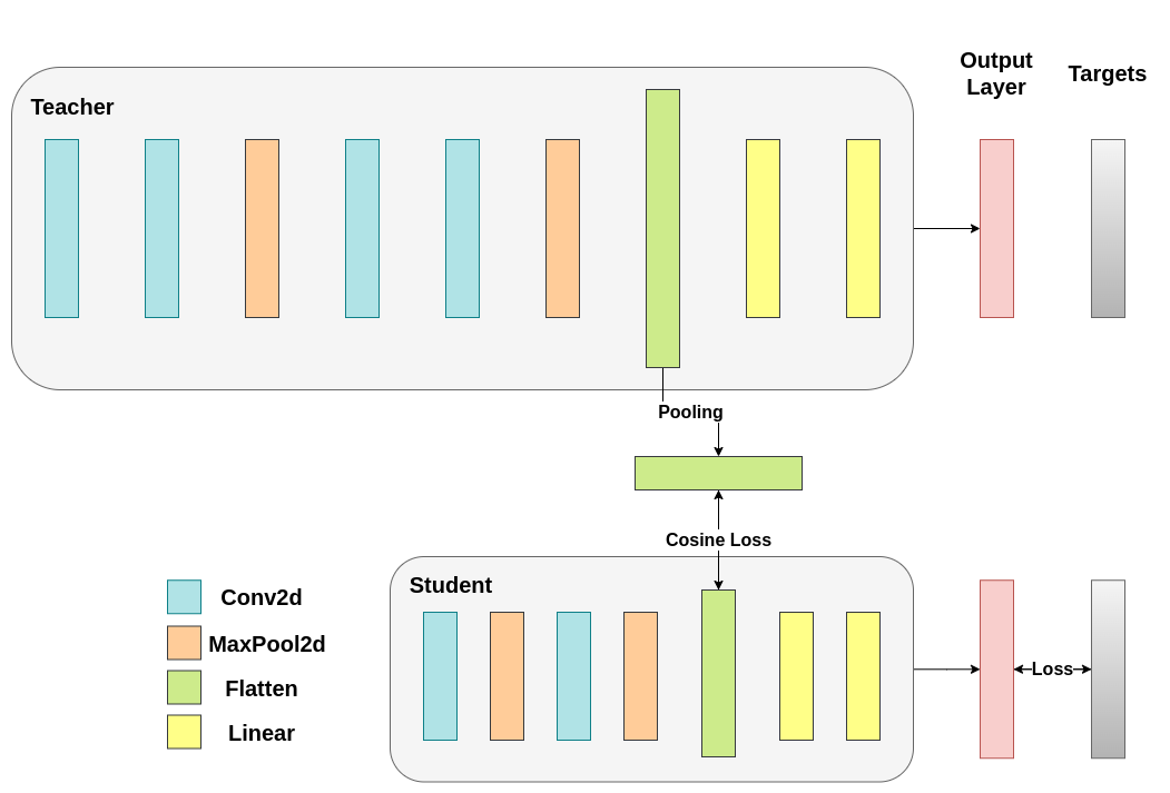
随意调整控制 softmax 函数柔软度的温度参数和损失系数。在神经网络中，很容易在主要目标中包含额外的损失函数，以实现更好的泛化等目标。让我们尝试为学生包含一个目标，但现在让我们关注它们的隐藏状态而不是它们的输出层。我们的目标是通过包含一个朴素的损失函数，将信息从教师的表示传递给学生，该函数的最小化意味着随后传递给分类器的扁平化向量随着损失的减少变得更加 相似。当然，教师不会更新其权重，因此最小化仅取决于学生的权重。这种方法背后的原理是，我们假设教师模型具有更好的内部表示，学生在没有外部干预的情况下不太可能达到这种表示，因此我们人为地推动学生模仿教师的内部表示。然而，这是否最终会帮助学生并不直接，因为推动轻量级网络达到这一点可能是一件好事，假设我们已经找到了导致更好测试准确性的内部表示，但它也可能是有害的，因为网络具有不同的架构，并且学生不具有与教师相同的学习能力。换句话说，这两个向量（学生的和教师的）没有理由逐个分量匹配。学生可以达到教师表示的排列，并且它同样高效。尽管如此，我们仍然可以进行快速实验来找出这种方法的影响。我们将使用 CosineEmbeddingLoss，其公式如下：

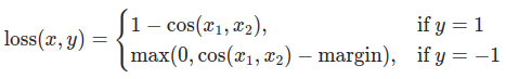
CosineEmbeddingLoss 的公式

显然，我们首先需要解决一个问题。当我们将蒸馏应用于输出层时，我们提到两个网络具有相同数量的神经元，等于类别的数量。然而，对于卷积层之后的层来说，情况并非如此。在这里，教师在最终卷积层扁平化后，神经元数量比学生多。我们的损失函数接受两个维度相同的向量作为输入，因此我们需要以某种方式匹配它们。我们将通过在教师的卷积层之后包含一个平均池化层来解决这个问题，以减少其维度以匹配学生的维度。

为了继续，我们将修改我们的模型类，或创建新的模型类。现在，前向函数不仅返回网络的 logits，还返回卷积层之后的扁平化隐藏表示。我们为修改后的教师包含了前面提到的池化。

class ModifiedDeepNNCosine(nn.Module):
    def __init__(self, num_classes=10):
        super(ModifiedDeepNNCosine, self).__init__()
        self.features = nn.Sequential(
            nn.Conv2d(3, 128, kernel_size=3, padding=1),
            nn.ReLU(),
            nn.Conv2d(128, 64, kernel_size=3, padding=1),
            nn.ReLU(),
            nn.MaxPool2d(kernel_size=2, stride=2),
            nn.Conv2d(64, 64, kernel_size=3, padding=1),
            nn.ReLU(),
            nn.Conv2d(64, 32, kernel_size=3, padding=1),
            nn.ReLU(),
            nn.MaxPool2d(kernel_size=2, stride=2),
        )
        self.classifier = nn.Sequential(
            nn.Linear(2048, 512),
            nn.ReLU(),
            nn.Dropout(0.1),
            nn.Linear(512, num_classes)
        )

    def forward(self, x):
        x = self.features(x)
        flattened_conv_output = torch.flatten(x, 1)
        x = self.classifier(flattened_conv_output)
        flattened_conv_output_after_pooling = torch.nn.functional.avg_pool1d(flattened_conv_output, 2)
        return x, flattened_conv_output_after_pooling

# Create a similar student class where we return a tuple. We do not apply pooling after flattening.
class ModifiedLightNNCosine(nn.Module):
    def __init__(self, num_classes=10):
        super(ModifiedLightNNCosine, self).__init__()
        self.features = nn.Sequential(
            nn.Conv2d(3, 16, kernel_size=3, padding=1),
            nn.ReLU(),
            nn.MaxPool2d(kernel_size=2, stride=2),
            nn.Conv2d(16, 16, kernel_size=3, padding=1),
            nn.ReLU(),
            nn.MaxPool2d(kernel_size=2, stride=2),
        )
        self.classifier = nn.Sequential(
            nn.Linear(1024, 256),
            nn.ReLU(),
            nn.Dropout(0.1),
            nn.Linear(256, num_classes)
        )

    def forward(self, x):
        x = self.features(x)
        flattened_conv_output = torch.flatten(x, 1)
        x = self.classifier(flattened_conv_output)
        return x, flattened_conv_output

# We do not have to train the modified deep network from scratch of course, we just load its weights from the trained instance
modified_nn_deep = ModifiedDeepNNCosine(num_classes=10).to(device)
modified_nn_deep.load_state_dict(nn_deep.state_dict())

# Once again ensure the norm of the first layer is the same for both networks
print("Norm of 1st layer for deep_nn:", torch.norm(nn_deep.features[0].weight).item())
print("Norm of 1st layer for modified_deep_nn:", torch.norm(modified_nn_deep.features[0].weight).item())

# Initialize a modified lightweight network with the same seed as our other lightweight instances. This will be trained from scratch to examine the effectiveness of cosine loss minimization.
torch.manual_seed(42)
modified_nn_light = ModifiedLightNNCosine(num_classes=10).to(device)
print("Norm of 1st layer:", torch.norm(modified_nn_light.features[0].weight).item())

Norm of 1st layer for deep_nn: 7.475808143615723
Norm of 1st layer for modified_deep_nn: 7.475808143615723
Norm of 1st layer: 2.327361822128296

自然，我们需要改变训练循环，因为现在模型返回一个元组 (logits, hidden_representation)。使用一个样本输入张量，我们可以打印它们的形状。

# Create a sample input tensor
sample_input = torch.randn(128, 3, 32, 32).to(device) # Batch size: 128, Filters: 3, Image size: 32x32

# Pass the input through the student
logits, hidden_representation = modified_nn_light(sample_input)

# Print the shapes of the tensors
print("Student logits shape:", logits.shape) # batch_size x total_classes
print("Student hidden representation shape:", hidden_representation.shape) # batch_size x hidden_representation_size

# Pass the input through the teacher
logits, hidden_representation = modified_nn_deep(sample_input)

# Print the shapes of the tensors
print("Teacher logits shape:", logits.shape) # batch_size x total_classes
print("Teacher hidden representation shape:", hidden_representation.shape) # batch_size x hidden_representation_size

Student logits shape: torch.Size([128, 10])
Student hidden representation shape: torch.Size([128, 1024])
Teacher logits shape: torch.Size([128, 10])
Teacher hidden representation shape: torch.Size([128, 1024])

在我们的例子中，hidden_representation_size 是 1024。这是学生最后一个卷积层的扁平化特征图，正如你所看到的，它是其分类器的输入。对于教师来说，它也是 1024，因为我们用 avg_pool1d 从 2048 实现了这一点。这里应用的损失只影响损失计算前学生的权重。换句话说，它不影响学生的分类器。修改后的训练循环如下：

在余弦损失最小化中，我们希望通过向学生返回梯度来最大化两个表示的余弦相似度：

def train_cosine_loss(teacher, student, train_loader, epochs, learning_rate, hidden_rep_loss_weight, ce_loss_weight, device):
    ce_loss = nn.CrossEntropyLoss()
    cosine_loss = nn.CosineEmbeddingLoss()
    optimizer = optim.Adam(student.parameters(), lr=learning_rate)

    teacher.to(device)
    student.to(device)
    teacher.eval()  # Teacher set to evaluation mode
    student.train() # Student to train mode

    for epoch in range(epochs):
        running_loss = 0.0
        for inputs, labels in train_loader:
            inputs, labels = inputs.to(device), labels.to(device)

            optimizer.zero_grad()

            # Forward pass with the teacher model and keep only the hidden representation
            with torch.no_grad():
                _, teacher_hidden_representation = teacher(inputs)

            # Forward pass with the student model
            student_logits, student_hidden_representation = student(inputs)

            # Calculate the cosine loss. Target is a vector of ones. From the loss formula above we can see that is the case where loss minimization leads to cosine similarity increase.
            hidden_rep_loss = cosine_loss(student_hidden_representation, teacher_hidden_representation, target=torch.ones(inputs.size(0)).to(device))

            # Calculate the true label loss
            label_loss = ce_loss(student_logits, labels)

            # Weighted sum of the two losses
            loss = hidden_rep_loss_weight * hidden_rep_loss + ce_loss_weight * label_loss

            loss.backward()
            optimizer.step()

            running_loss += loss.item()

        print(f"Epoch {epoch+1}/{epochs}, Loss: {running_loss / len(train_loader)}")

出于同样的原因，我们需要修改我们的测试函数。这里我们忽略模型返回的隐藏表示。

def test_multiple_outputs(model, test_loader, device):
    model.to(device)
    model.eval()

    correct = 0
    total = 0

    with torch.no_grad():
        for inputs, labels in test_loader:
            inputs, labels = inputs.to(device), labels.to(device)

            outputs, _ = model(inputs) # Disregard the second tensor of the tuple
            _, predicted = torch.max(outputs.data, 1)

            total += labels.size(0)
            correct += (predicted == labels).sum().item()

    accuracy = 100 * correct / total
    print(f"Test Accuracy: {accuracy:.2f}%")
    return accuracy

在这种情况下，我们可以很容易地将知识蒸馏和余弦损失最小化都包含在同一个函数中。在师生范式中，结合多种方法以获得更好的性能是很常见的。目前，我们可以进行一个简单的训练-测试会话。

# Train and test the lightweight network with cross entropy loss
train_cosine_loss(teacher=modified_nn_deep, student=modified_nn_light, train_loader=train_loader, epochs=10, learning_rate=0.001, hidden_rep_loss_weight=0.25, ce_loss_weight=0.75, device=device)
test_accuracy_light_ce_and_cosine_loss = test_multiple_outputs(modified_nn_light, test_loader, device)

Epoch 1/10, Loss: 1.3035651055138435
Epoch 2/10, Loss: 1.0732358320594748
Epoch 3/10, Loss: 0.9711669814556151
Epoch 4/10, Loss: 0.894416183919248
Epoch 5/10, Loss: 0.8372297442477682
Epoch 6/10, Loss: 0.7941221222853112
Epoch 7/10, Loss: 0.7529998520756012
Epoch 8/10, Loss: 0.716936968171688
Epoch 9/10, Loss: 0.6803364531158487
Epoch 10/10, Loss: 0.653171255003156
Test Accuracy: 70.15%

中间回归器运行

我们的朴素最小化不能保证更好的结果，原因有几个，其中之一是向量的维度。余弦相似度对于高维向量通常比欧几里得距离效果更好，但我们处理的是每个具有 1024 个分量的向量，因此提取有意义的相似性要困难得多。此外，正如我们所提到的，将教师和学生的隐藏表示推向匹配是不受理论支持的。没有充分的理由说明我们为什么要追求这些向量的 1:1 匹配。我们将提供一个最终的训练干预示例，通过包含一个名为回归器的额外网络。目标是首先提取卷积层之后教师的特征图，然后提取卷积层之后学生的特征图，最后尝试匹配这些特征图。然而，这次我们将在网络之间引入一个回归器，以促进匹配过程。回归器将是可训练的，理想情况下将比我们朴素的余弦损失最小化方案做得更好。它的主要作用是匹配这些特征图的维度，以便我们可以正确定义教师和学生之间的损失函数。定义这样的损失函数提供了一条教学“路径”，它基本上是一个反向传播梯度的流，这些梯度将改变学生的权重。关注我们原始网络中每个分类器之前卷积层的输出，我们有以下形状

# Pass the sample input only from the convolutional feature extractor
convolutional_fe_output_student = nn_light.features(sample_input)
convolutional_fe_output_teacher = nn_deep.features(sample_input)

# Print their shapes
print("Student's feature extractor output shape: ", convolutional_fe_output_student.shape)
print("Teacher's feature extractor output shape: ", convolutional_fe_output_teacher.shape)

Student's feature extractor output shape:  torch.Size([128, 16, 8, 8])
Teacher's feature extractor output shape:  torch.Size([128, 32, 8, 8])

教师有 32 个滤波器，学生有 16 个滤波器。我们将包含一个可训练层，将学生的特征图转换为教师的特征图形状。实际上，我们修改轻量级类，使其在中间回归器之后返回隐藏状态，该回归器匹配卷积特征图的大小，而教师类则返回最终卷积层的输出，不进行池化或扁平化。

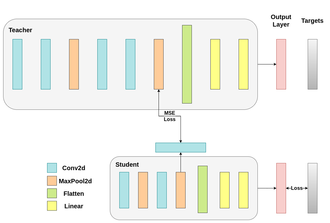
可训练层匹配中间张量的形状，并且均方误差（MSE）被正确定义：

class ModifiedDeepNNRegressor(nn.Module):
    def __init__(self, num_classes=10):
        super(ModifiedDeepNNRegressor, self).__init__()
        self.features = nn.Sequential(
            nn.Conv2d(3, 128, kernel_size=3, padding=1),
            nn.ReLU(),
            nn.Conv2d(128, 64, kernel_size=3, padding=1),
            nn.ReLU(),
            nn.MaxPool2d(kernel_size=2, stride=2),
            nn.Conv2d(64, 64, kernel_size=3, padding=1),
            nn.ReLU(),
            nn.Conv2d(64, 32, kernel_size=3, padding=1),
            nn.ReLU(),
            nn.MaxPool2d(kernel_size=2, stride=2),
        )
        self.classifier = nn.Sequential(
            nn.Linear(2048, 512),
            nn.ReLU(),
            nn.Dropout(0.1),
            nn.Linear(512, num_classes)
        )

    def forward(self, x):
        x = self.features(x)
        conv_feature_map = x
        x = torch.flatten(x, 1)
        x = self.classifier(x)
        return x, conv_feature_map

class ModifiedLightNNRegressor(nn.Module):
    def __init__(self, num_classes=10):
        super(ModifiedLightNNRegressor, self).__init__()
        self.features = nn.Sequential(
            nn.Conv2d(3, 16, kernel_size=3, padding=1),
            nn.ReLU(),
            nn.MaxPool2d(kernel_size=2, stride=2),
            nn.Conv2d(16, 16, kernel_size=3, padding=1),
            nn.ReLU(),
            nn.MaxPool2d(kernel_size=2, stride=2),
        )
        # Include an extra regressor (in our case linear)
        self.regressor = nn.Sequential(
            nn.Conv2d(16, 32, kernel_size=3, padding=1)
        )
        self.classifier = nn.Sequential(
            nn.Linear(1024, 256),
            nn.ReLU(),
            nn.Dropout(0.1),
            nn.Linear(256, num_classes)
        )

    def forward(self, x):
        x = self.features(x)
        regressor_output = self.regressor(x)
        x = torch.flatten(x, 1)
        x = self.classifier(x)
        return x, regressor_output

之后，我们必须再次更新我们的训练循环。这次，我们提取学生的回归器输出，教师的特征图，计算这些张量的 MSE（它们具有完全相同的形状，因此定义正确），并根据该损失反向传播梯度，此外还有分类任务的常规交叉熵损失。

def train_mse_loss(teacher, student, train_loader, epochs, learning_rate, feature_map_weight, ce_loss_weight, device):
    ce_loss = nn.CrossEntropyLoss()
    mse_loss = nn.MSELoss()
    optimizer = optim.Adam(student.parameters(), lr=learning_rate)

    teacher.to(device)
    student.to(device)
    teacher.eval()  # Teacher set to evaluation mode
    student.train() # Student to train mode

    for epoch in range(epochs):
        running_loss = 0.0
        for inputs, labels in train_loader:
            inputs, labels = inputs.to(device), labels.to(device)

            optimizer.zero_grad()

            # Again ignore teacher logits
            with torch.no_grad():
                _, teacher_feature_map = teacher(inputs)

            # Forward pass with the student model
            student_logits, regressor_feature_map = student(inputs)

            # Calculate the loss
            hidden_rep_loss = mse_loss(regressor_feature_map, teacher_feature_map)

            # Calculate the true label loss
            label_loss = ce_loss(student_logits, labels)

            # Weighted sum of the two losses
            loss = feature_map_weight * hidden_rep_loss + ce_loss_weight * label_loss

            loss.backward()
            optimizer.step()

            running_loss += loss.item()

        print(f"Epoch {epoch+1}/{epochs}, Loss: {running_loss / len(train_loader)}")

# Notice how our test function remains the same here with the one we used in our previous case. We only care about the actual outputs because we measure accuracy.

# Initialize a ModifiedLightNNRegressor
torch.manual_seed(42)
modified_nn_light_reg = ModifiedLightNNRegressor(num_classes=10).to(device)

# We do not have to train the modified deep network from scratch of course, we just load its weights from the trained instance
modified_nn_deep_reg = ModifiedDeepNNRegressor(num_classes=10).to(device)
modified_nn_deep_reg.load_state_dict(nn_deep.state_dict())

# Train and test once again
train_mse_loss(teacher=modified_nn_deep_reg, student=modified_nn_light_reg, train_loader=train_loader, epochs=10, learning_rate=0.001, feature_map_weight=0.25, ce_loss_weight=0.75, device=device)
test_accuracy_light_ce_and_mse_loss = test_multiple_outputs(modified_nn_light_reg, test_loader, device)

Epoch 1/10, Loss: 1.7514760850945397
Epoch 2/10, Loss: 1.3703956210704715
Epoch 3/10, Loss: 1.2287705946151557
Epoch 4/10, Loss: 1.1349974331038688
Epoch 5/10, Loss: 1.057304141771458
Epoch 6/10, Loss: 0.9946642374748464
Epoch 7/10, Loss: 0.9410008506091965
Epoch 8/10, Loss: 0.8928298277928092
Epoch 9/10, Loss: 0.8475199328054248
Epoch 10/10, Loss: 0.8124411052755077
Test Accuracy: 70.45%

最终的方法预计会比 CosineLoss 效果更好，因为现在我们在教师和学生之间引入了一个可训练层，这给了学生在学习时一定的灵活度，而不是强制学生复制教师的表示。引入额外的网络是基于提示的蒸馏背后的思想。

print(f"Teacher accuracy: {test_accuracy_deep:.2f}%")
print(f"Student accuracy without teacher: {test_accuracy_light_ce:.2f}%")
print(f"Student accuracy with CE + KD: {test_accuracy_light_ce_and_kd:.2f}%")
print(f"Student accuracy with CE + CosineLoss: {test_accuracy_light_ce_and_cosine_loss:.2f}%")
print(f"Student accuracy with CE + RegressorMSE: {test_accuracy_light_ce_and_mse_loss:.2f}%")

Teacher accuracy: 74.58%
Student accuracy without teacher: 70.03%
Student accuracy with CE + KD: 71.02%
Student accuracy with CE + CosineLoss: 70.15%
Student accuracy with CE + RegressorMSE: 70.45%

结论

上述方法都不会增加网络的参数数量或推理时间，因此性能提升带来的代价只是在训练期间计算梯度。在机器学习应用中，我们主要关心推理时间，因为训练发生在模型部署之前。如果我们的轻量级模型仍然太重而无法部署，我们可以应用不同的想法，例如训练后量化。额外的损失可以应用于许多任务，而不仅仅是分类，您可以尝试系数、温度或神经元数量等量。请随意调整上述教程中的任何数字，但请记住，如果您更改神经元/滤波器的数量，则可能会发生形状不匹配。

欲了解更多信息，请参阅

• Hinton, G., Vinyals, O., Dean, J.: 神经网络中的知识蒸馏. 在: 神经网络信息处理系统深度学习研讨会 (2015)

• Romero, A., Ballas, N., Kahou, S.E., Chassang, A., Gatta, C., Bengio, Y.: Fitnets: 薄型深层网络的提示. 在: 国际学习表示大会论文集 (2015)