


注意
转到末尾 下载完整的示例代码。
计算机视觉迁移学习教程#
创建日期: 2017 年 3 月 24 日 | 最后更新: 2025 年 1 月 27 日 | 最后验证: 2024 年 11 月 5 日
在本教程中,您将学习如何使用迁移学习来训练用于图像分类的卷积神经网络。您可以在 cs231n 笔记 中阅读更多关于迁移学习的内容。
引用这些笔记,
实际上,很少有人从头开始训练整个卷积网络(使用随机初始化),因为拥有足够大的数据集相对罕见。相反,通常的做法是在非常大的数据集(例如 ImageNet,包含 120 万张图像和 1000 个类别)上预训练一个卷积网络,然后将该卷积网络用作初始化或固定的特征提取器来处理感兴趣的任务。
这两种主要的迁移学习场景如下所示:
微调卷积网络:我们不使用随机初始化,而是用预训练网络(例如在 ImageNet 1000 数据集上训练的网络)初始化网络。其余的训练过程照常进行。
将卷积网络作为固定的特征提取器:在这里,我们将冻结网络中除最后一个全连接层之外的所有层的权重。最后一个全连接层被一个新的具有随机权重的层替换,并且只有这一层被训练。
# License: BSD
# Author: Sasank Chilamkurthy

import torch
import torch.nn as nn
import torch.optim as optim
from torch.optim import lr_scheduler
import torch.backends.cudnn as cudnn
import numpy as np
import torchvision
from torchvision import datasets, models, transforms
import matplotlib.pyplot as plt
import time
import os
from PIL import Image
from tempfile import TemporaryDirectory

cudnn.benchmark = True
plt.ion()   # interactive mode
<contextlib.ExitStack object at 0x7f33e6095150>
加载数据#
我们将使用 torchvision 和 torch.utils.data 包来加载数据。
今天我们要解决的问题是训练一个模型来分类蚂蚁和蜜蜂。我们有大约 120 张蚂蚁和蜜蜂的训练图像。每种类别有 75 张验证图像。通常,如果从头开始训练,这个数据集太小,无法进行泛化。由于我们正在使用迁移学习,我们应该能够进行相当好的泛化。
该数据集是 ImageNet 的一个非常小的子集。
注意
从 这里 下载数据,并将其解压到当前目录。
# Data augmentation and normalization for training
# Just normalization for validation
data_transforms = {
    'train': transforms.Compose([
        transforms.RandomResizedCrop(224),
        transforms.RandomHorizontalFlip(),
        transforms.ToTensor(),
        transforms.Normalize([0.485, 0.456, 0.406], [0.229, 0.224, 0.225])
    ]),
    'val': transforms.Compose([
        transforms.Resize(256),
        transforms.CenterCrop(224),
        transforms.ToTensor(),
        transforms.Normalize([0.485, 0.456, 0.406], [0.229, 0.224, 0.225])
    ]),
}

data_dir = 'data/hymenoptera_data'
image_datasets = {x: datasets.ImageFolder(os.path.join(data_dir, x),
                                          data_transforms[x])
                  for x in ['train', 'val']}
dataloaders = {x: torch.utils.data.DataLoader(image_datasets[x], batch_size=4,
                                             shuffle=True, num_workers=4)
              for x in ['train', 'val']}
dataset_sizes = {x: len(image_datasets[x]) for x in ['train', 'val']}
class_names = image_datasets['train'].classes

# We want to be able to train our model on an `accelerator <https://pytorch.ac.cn/docs/stable/torch.html#accelerators>`__
# such as CUDA, MPS, MTIA, or XPU. If the current accelerator is available, we will use it. Otherwise, we use the CPU.

device = torch.accelerator.current_accelerator().type if torch.accelerator.is_available() else "cpu"
print(f"Using {device} device")
Using cuda device
可视化几张图片#
让我们可视化几张训练图像,以便了解数据增强。
def imshow(inp, title=None):
    """Display image for Tensor."""
    inp = inp.numpy().transpose((1, 2, 0))
    mean = np.array([0.485, 0.456, 0.406])
    std = np.array([0.229, 0.224, 0.225])
    inp = std * inp + mean
    inp = np.clip(inp, 0, 1)
    plt.imshow(inp)
    if title is not None:
        plt.title(title)
    plt.pause(0.001)  # pause a bit so that plots are updated


# Get a batch of training data
inputs, classes = next(iter(dataloaders['train']))

# Make a grid from batch
out = torchvision.utils.make_grid(inputs)

imshow(out, title=[class_names[x] for x in classes])
![['ants', 'ants', 'bees', 'ants']](../_images/sphx_glr_transfer_learning_tutorial_001.png)
训练模型#
现在,让我们编写一个通用的函数来训练模型。在这里,我们将演示
学习率调度
保存最佳模型
在接下来的内容中,参数 scheduler 是来自 torch.optim.lr_scheduler 的 LR 调度器对象。
def train_model(model, criterion, optimizer, scheduler, num_epochs=25):
    since = time.time()

    # Create a temporary directory to save training checkpoints
    with TemporaryDirectory() as tempdir:
        best_model_params_path = os.path.join(tempdir, 'best_model_params.pt')

        torch.save(model.state_dict(), best_model_params_path)
        best_acc = 0.0

        for epoch in range(num_epochs):
            print(f'Epoch {epoch}/{num_epochs - 1}')
            print('-' * 10)

            # Each epoch has a training and validation phase
            for phase in ['train', 'val']:
                if phase == 'train':
                    model.train()  # Set model to training mode
                else:
                    model.eval()   # Set model to evaluate mode

                running_loss = 0.0
                running_corrects = 0

                # Iterate over data.
                for inputs, labels in dataloaders[phase]:
                    inputs = inputs.to(device)
                    labels = labels.to(device)

                    # zero the parameter gradients
                    optimizer.zero_grad()

                    # forward
                    # track history if only in train
                    with torch.set_grad_enabled(phase == 'train'):
                        outputs = model(inputs)
                        _, preds = torch.max(outputs, 1)
                        loss = criterion(outputs, labels)

                        # backward + optimize only if in training phase
                        if phase == 'train':
                            loss.backward()
                            optimizer.step()

                    # statistics
                    running_loss += loss.item() * inputs.size(0)
                    running_corrects += torch.sum(preds == labels.data)
                if phase == 'train':
                    scheduler.step()

                epoch_loss = running_loss / dataset_sizes[phase]
                epoch_acc = running_corrects.double() / dataset_sizes[phase]

                print(f'{phase} Loss: {epoch_loss:.4f} Acc: {epoch_acc:.4f}')

                # deep copy the model
                if phase == 'val' and epoch_acc > best_acc:
                    best_acc = epoch_acc
                    torch.save(model.state_dict(), best_model_params_path)

            print()

        time_elapsed = time.time() - since
        print(f'Training complete in {time_elapsed // 60:.0f}m {time_elapsed % 60:.0f}s')
        print(f'Best val Acc: {best_acc:4f}')

        # load best model weights
        model.load_state_dict(torch.load(best_model_params_path, weights_only=True))
    return model
可视化模型预测#
用于显示几张图像预测的通用函数
def visualize_model(model, num_images=6):
    was_training = model.training
    model.eval()
    images_so_far = 0
    fig = plt.figure()

    with torch.no_grad():
        for i, (inputs, labels) in enumerate(dataloaders['val']):
            inputs = inputs.to(device)
            labels = labels.to(device)

            outputs = model(inputs)
            _, preds = torch.max(outputs, 1)

            for j in range(inputs.size()[0]):
                images_so_far += 1
                ax = plt.subplot(num_images//2, 2, images_so_far)
                ax.axis('off')
                ax.set_title(f'predicted: {class_names[preds[j]]}')
                imshow(inputs.cpu().data[j])

                if images_so_far == num_images:
                    model.train(mode=was_training)
                    return
        model.train(mode=was_training)
微调卷积网络#
加载预训练模型并重置最后的全连接层。
model_ft = models.resnet18(weights='IMAGENET1K_V1')
num_ftrs = model_ft.fc.in_features
# Here the size of each output sample is set to 2.
# Alternatively, it can be generalized to ``nn.Linear(num_ftrs, len(class_names))``.
model_ft.fc = nn.Linear(num_ftrs, 2)

model_ft = model_ft.to(device)

criterion = nn.CrossEntropyLoss()

# Observe that all parameters are being optimized
optimizer_ft = optim.SGD(model_ft.parameters(), lr=0.001, momentum=0.9)

# Decay LR by a factor of 0.1 every 7 epochs
exp_lr_scheduler = lr_scheduler.StepLR(optimizer_ft, step_size=7, gamma=0.1)
Downloading: "https://download.pytorch.org/models/resnet18-f37072fd.pth" to /var/lib/ci-user/.cache/torch/hub/checkpoints/resnet18-f37072fd.pth

  0%|          | 0.00/44.7M [00:00<?, ?B/s]
 86%|████████▌ | 38.2M/44.7M [00:00<00:00, 401MB/s]
100%|██████████| 44.7M/44.7M [00:00<00:00, 405MB/s]
训练和评估#
在 CPU 上大约需要 15-25 分钟。但在 GPU 上,则不到一分钟。
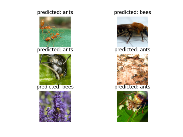
model_ft = train_model(model_ft, criterion, optimizer_ft, exp_lr_scheduler,
                       num_epochs=25)
Epoch 0/24
----------
train Loss: 0.6373 Acc: 0.6516
val Loss: 0.2572 Acc: 0.9085

Epoch 1/24
----------
train Loss: 0.5740 Acc: 0.7623
val Loss: 0.2817 Acc: 0.8824

Epoch 2/24
----------
train Loss: 0.6096 Acc: 0.7992
val Loss: 0.3793 Acc: 0.8562

Epoch 3/24
----------
train Loss: 0.5331 Acc: 0.7828
val Loss: 0.5794 Acc: 0.7778

Epoch 4/24
----------
train Loss: 0.4826 Acc: 0.7992
val Loss: 0.2825 Acc: 0.8693

Epoch 5/24
----------
train Loss: 0.4198 Acc: 0.8443
val Loss: 0.3402 Acc: 0.8497

Epoch 6/24
----------
train Loss: 0.5800 Acc: 0.7992
val Loss: 0.3691 Acc: 0.8627

Epoch 7/24
----------
train Loss: 0.4223 Acc: 0.8238
val Loss: 0.2912 Acc: 0.9020

Epoch 8/24
----------
train Loss: 0.3087 Acc: 0.8607
val Loss: 0.3402 Acc: 0.8497

Epoch 9/24
----------
train Loss: 0.3541 Acc: 0.8484
val Loss: 0.3100 Acc: 0.9020

Epoch 10/24
----------
train Loss: 0.3052 Acc: 0.8443
val Loss: 0.2970 Acc: 0.9020

Epoch 11/24
----------
train Loss: 0.3013 Acc: 0.8648
val Loss: 0.2608 Acc: 0.9216

Epoch 12/24
----------
train Loss: 0.3507 Acc: 0.8607
val Loss: 0.2229 Acc: 0.9216

Epoch 13/24
----------
train Loss: 0.2282 Acc: 0.8852
val Loss: 0.2335 Acc: 0.9150

Epoch 14/24
----------
train Loss: 0.2732 Acc: 0.8811
val Loss: 0.2603 Acc: 0.8954

Epoch 15/24
----------
train Loss: 0.2815 Acc: 0.8934
val Loss: 0.2593 Acc: 0.8954

Epoch 16/24
----------
train Loss: 0.3011 Acc: 0.8648
val Loss: 0.2444 Acc: 0.9020

Epoch 17/24
----------
train Loss: 0.2845 Acc: 0.8648
val Loss: 0.2330 Acc: 0.9150

Epoch 18/24
----------
train Loss: 0.2321 Acc: 0.9057
val Loss: 0.2444 Acc: 0.9085

Epoch 19/24
----------
train Loss: 0.2707 Acc: 0.8730
val Loss: 0.2563 Acc: 0.9020

Epoch 20/24
----------
train Loss: 0.3090 Acc: 0.8852
val Loss: 0.2208 Acc: 0.9216

Epoch 21/24
----------
train Loss: 0.3351 Acc: 0.8566
val Loss: 0.2936 Acc: 0.8954

Epoch 22/24
----------
train Loss: 0.2792 Acc: 0.8770
val Loss: 0.2424 Acc: 0.9020

Epoch 23/24
----------
train Loss: 0.2974 Acc: 0.8648
val Loss: 0.2344 Acc: 0.9085

Epoch 24/24
----------
train Loss: 0.3274 Acc: 0.8689
val Loss: 0.2757 Acc: 0.8824

Training complete in 0m 36s
Best val Acc: 0.921569
visualize_model(model_ft)
将卷积网络作为固定的特征提取器#
在这里,我们需要冻结除了最后一层之外的所有网络。我们需要将 requires_grad = False 来冻结参数,以便在 backward() 中不计算梯度。
您可以在文档 这里 中阅读更多关于此内容的信息。
model_conv = torchvision.models.resnet18(weights='IMAGENET1K_V1')
for param in model_conv.parameters():
    param.requires_grad = False

# Parameters of newly constructed modules have requires_grad=True by default
num_ftrs = model_conv.fc.in_features
model_conv.fc = nn.Linear(num_ftrs, 2)

model_conv = model_conv.to(device)

criterion = nn.CrossEntropyLoss()

# Observe that only parameters of final layer are being optimized as
# opposed to before.
optimizer_conv = optim.SGD(model_conv.fc.parameters(), lr=0.001, momentum=0.9)

# Decay LR by a factor of 0.1 every 7 epochs
exp_lr_scheduler = lr_scheduler.StepLR(optimizer_conv, step_size=7, gamma=0.1)
训练和评估#
在 CPU 上,这大约需要前一种情况一半的时间。这是预期的,因为大多数网络不需要计算梯度。但是,前向传播仍然需要计算。
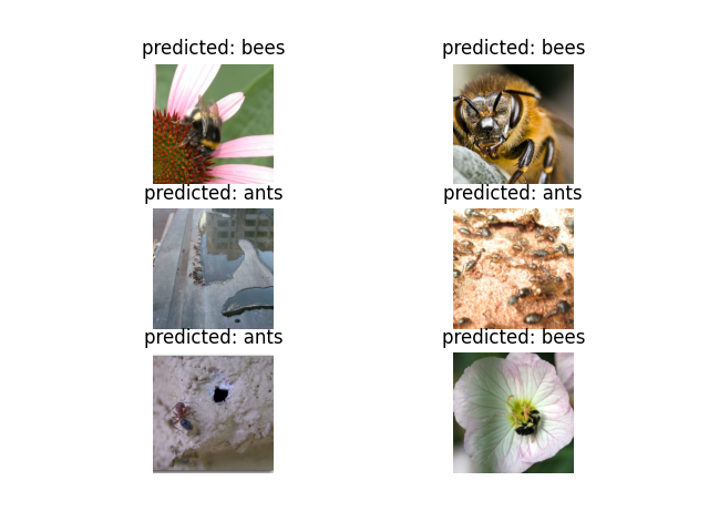
model_conv = train_model(model_conv, criterion, optimizer_conv,
                         exp_lr_scheduler, num_epochs=25)
Epoch 0/24
----------
train Loss: 0.6005 Acc: 0.6516
val Loss: 0.3484 Acc: 0.8497

Epoch 1/24
----------
train Loss: 0.4055 Acc: 0.8074
val Loss: 0.1546 Acc: 0.9477

Epoch 2/24
----------
train Loss: 0.3788 Acc: 0.8238
val Loss: 0.2740 Acc: 0.8889

Epoch 3/24
----------
train Loss: 0.4735 Acc: 0.8074
val Loss: 0.1895 Acc: 0.9346

Epoch 4/24
----------
train Loss: 0.4034 Acc: 0.8402
val Loss: 0.1625 Acc: 0.9346

Epoch 5/24
----------
train Loss: 0.3522 Acc: 0.8443
val Loss: 0.1662 Acc: 0.9542

Epoch 6/24
----------
train Loss: 0.5148 Acc: 0.7664
val Loss: 0.5580 Acc: 0.7974

Epoch 7/24
----------
train Loss: 0.5086 Acc: 0.7910
val Loss: 0.1755 Acc: 0.9542

Epoch 8/24
----------
train Loss: 0.3373 Acc: 0.8279
val Loss: 0.2159 Acc: 0.9412

Epoch 9/24
----------
train Loss: 0.3281 Acc: 0.8525
val Loss: 0.1755 Acc: 0.9477

Epoch 10/24
----------
train Loss: 0.3662 Acc: 0.8648
val Loss: 0.1813 Acc: 0.9542

Epoch 11/24
----------
train Loss: 0.3764 Acc: 0.8279
val Loss: 0.1766 Acc: 0.9477

Epoch 12/24
----------
train Loss: 0.3467 Acc: 0.8361
val Loss: 0.2039 Acc: 0.9412

Epoch 13/24
----------
train Loss: 0.2729 Acc: 0.8730
val Loss: 0.1693 Acc: 0.9542

Epoch 14/24
----------
train Loss: 0.4085 Acc: 0.8156
val Loss: 0.1752 Acc: 0.9542

Epoch 15/24
----------
train Loss: 0.3271 Acc: 0.8852
val Loss: 0.1763 Acc: 0.9542

Epoch 16/24
----------
train Loss: 0.3405 Acc: 0.8402
val Loss: 0.1858 Acc: 0.9608

Epoch 17/24
----------
train Loss: 0.2761 Acc: 0.9016
val Loss: 0.1821 Acc: 0.9542

Epoch 18/24
----------
train Loss: 0.3294 Acc: 0.8320
val Loss: 0.2104 Acc: 0.9412

Epoch 19/24
----------
train Loss: 0.2609 Acc: 0.8893
val Loss: 0.1764 Acc: 0.9542

Epoch 20/24
----------
train Loss: 0.3810 Acc: 0.8443
val Loss: 0.1840 Acc: 0.9477

Epoch 21/24
----------
train Loss: 0.3185 Acc: 0.8525
val Loss: 0.1795 Acc: 0.9477

Epoch 22/24
----------
train Loss: 0.3281 Acc: 0.8811
val Loss: 0.2054 Acc: 0.9412

Epoch 23/24
----------
train Loss: 0.3509 Acc: 0.8443
val Loss: 0.2059 Acc: 0.9412

Epoch 24/24
----------
train Loss: 0.3028 Acc: 0.8443
val Loss: 0.1932 Acc: 0.9542

Training complete in 0m 28s
Best val Acc: 0.960784
visualize_model(model_conv)

plt.ioff()
plt.show()
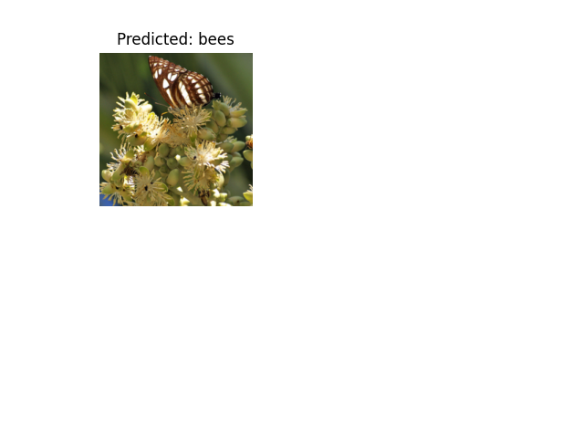
在自定义图像上进行推理#
使用训练好的模型在自定义图像上进行预测,并可视化预测的类别标签以及图像。
def visualize_model_predictions(model,img_path):
    was_training = model.training
    model.eval()

    img = Image.open(img_path)
    img = data_transforms['val'](img)
    img = img.unsqueeze(0)
    img = img.to(device)

    with torch.no_grad():
        outputs = model(img)
        _, preds = torch.max(outputs, 1)

        ax = plt.subplot(2,2,1)
        ax.axis('off')
        ax.set_title(f'Predicted: {class_names[preds[0]]}')
        imshow(img.cpu().data[0])

        model.train(mode=was_training)
visualize_model_predictions(
    model_conv,
    img_path='data/hymenoptera_data/val/bees/72100438_73de9f17af.jpg'
)

plt.ioff()
plt.show()
进一步学习#
如果您想了解更多关于迁移学习的应用,请查看我们的 计算机视觉量化迁移学习教程。
脚本总运行时间: (1 分钟 6.486 秒)
