intermediate/spatial_transformer_tutorial

在 Google Colab 中运行
Colab

下载 Notebook
Notebook

在 GitHub 上查看
GitHub
注意
转到末尾 下载完整的示例代码。
空间变换网络教程#
创建于:2017年11月08日 | 最后更新:2024年01月19日 | 最后验证:2024年11月05日
作者: Ghassen HAMROUNI

在本教程中,您将学习如何使用一种称为空间变换网络的视觉注意力机制来增强您的网络。您可以阅读更多关于空间变换网络的信息,请参阅 DeepMind 论文
空间变换网络是对任何空间变换的可微分注意力的泛化。空间变换网络(简称 STN)允许神经网络学习如何对输入图像执行空间变换,以增强模型的几何不变性。例如,它可以裁剪感兴趣的区域,缩放和校正图像的方向。这可能是一个有用的机制,因为卷积神经网络(CNN)对旋转、缩放以及更一般的仿射变换不是不变的。
STN 的一个优点是,只需进行很少的修改就可以将其插入任何现有的 CNN 中。
# License: BSD
# Author: Ghassen Hamrouni

import torch
import torch.nn as nn
import torch.nn.functional as F
import torch.optim as optim
import torchvision
from torchvision import datasets, transforms
import matplotlib.pyplot as plt
import numpy as np

plt.ion()   # interactive mode
<contextlib.ExitStack object at 0x7f2cfd4906d0>
加载数据#
在这篇文章中,我们尝试使用经典的 MNIST 数据集。使用带有空间变换网络的标准卷积网络。
from six.moves import urllib
opener = urllib.request.build_opener()
opener.addheaders = [('User-agent', 'Mozilla/5.0')]
urllib.request.install_opener(opener)

device = torch.device("cuda" if torch.cuda.is_available() else "cpu")

# Training dataset
train_loader = torch.utils.data.DataLoader(
    datasets.MNIST(root='.', train=True, download=True,
                   transform=transforms.Compose([
                       transforms.ToTensor(),
                       transforms.Normalize((0.1307,), (0.3081,))
                   ])), batch_size=64, shuffle=True, num_workers=4)
# Test dataset
test_loader = torch.utils.data.DataLoader(
    datasets.MNIST(root='.', train=False, transform=transforms.Compose([
        transforms.ToTensor(),
        transforms.Normalize((0.1307,), (0.3081,))
    ])), batch_size=64, shuffle=True, num_workers=4)
  0%|          | 0.00/9.91M [00:00<?, ?B/s]
100%|██████████| 9.91M/9.91M [00:00<00:00, 148MB/s]

  0%|          | 0.00/28.9k [00:00<?, ?B/s]
100%|██████████| 28.9k/28.9k [00:00<00:00, 21.2MB/s]

  0%|          | 0.00/1.65M [00:00<?, ?B/s]
100%|██████████| 1.65M/1.65M [00:00<00:00, 293MB/s]

  0%|          | 0.00/4.54k [00:00<?, ?B/s]
100%|██████████| 4.54k/4.54k [00:00<00:00, 28.0MB/s]
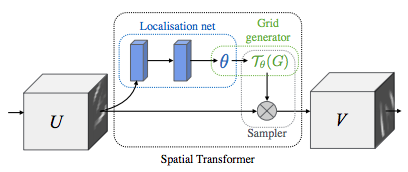
描绘空间变换网络#
空间变换网络归结为三个主要组成部分:
定位网络是一个常规的 CNN,用于回归变换参数。变换不是从数据集中显式学习的,而是网络自动学习增强全局准确性的空间变换。
网格生成器在输入图像中为输出图像的每个像素生成一个坐标网格。
采样器使用变换的参数并将其应用于输入图像。
注意
我们需要最新版本的 PyTorch,其中包含 affine_grid 和 grid_sample 模块。
class Net(nn.Module):
    def __init__(self):
        super(Net, self).__init__()
        self.conv1 = nn.Conv2d(1, 10, kernel_size=5)
        self.conv2 = nn.Conv2d(10, 20, kernel_size=5)
        self.conv2_drop = nn.Dropout2d()
        self.fc1 = nn.Linear(320, 50)
        self.fc2 = nn.Linear(50, 10)

        # Spatial transformer localization-network
        self.localization = nn.Sequential(
            nn.Conv2d(1, 8, kernel_size=7),
            nn.MaxPool2d(2, stride=2),
            nn.ReLU(True),
            nn.Conv2d(8, 10, kernel_size=5),
            nn.MaxPool2d(2, stride=2),
            nn.ReLU(True)
        )

        # Regressor for the 3 * 2 affine matrix
        self.fc_loc = nn.Sequential(
            nn.Linear(10 * 3 * 3, 32),
            nn.ReLU(True),
            nn.Linear(32, 3 * 2)
        )

        # Initialize the weights/bias with identity transformation
        self.fc_loc[2].weight.data.zero_()
        self.fc_loc[2].bias.data.copy_(torch.tensor([1, 0, 0, 0, 1, 0], dtype=torch.float))

    # Spatial transformer network forward function
    def stn(self, x):
        xs = self.localization(x)
        xs = xs.view(-1, 10 * 3 * 3)
        theta = self.fc_loc(xs)
        theta = theta.view(-1, 2, 3)

        grid = F.affine_grid(theta, x.size())
        x = F.grid_sample(x, grid)

        return x

    def forward(self, x):
        # transform the input
        x = self.stn(x)

        # Perform the usual forward pass
        x = F.relu(F.max_pool2d(self.conv1(x), 2))
        x = F.relu(F.max_pool2d(self.conv2_drop(self.conv2(x)), 2))
        x = x.view(-1, 320)
        x = F.relu(self.fc1(x))
        x = F.dropout(x, training=self.training)
        x = self.fc2(x)
        return F.log_softmax(x, dim=1)


model = Net().to(device)
训练模型#
现在,我们将使用 SGD 算法来训练模型。网络以监督方式学习分类任务。同时,模型以端到端的方式自动学习 STN。
optimizer = optim.SGD(model.parameters(), lr=0.01)


def train(epoch):
    model.train()
    for batch_idx, (data, target) in enumerate(train_loader):
        data, target = data.to(device), target.to(device)

        optimizer.zero_grad()
        output = model(data)
        loss = F.nll_loss(output, target)
        loss.backward()
        optimizer.step()
        if batch_idx % 500 == 0:
            print('Train Epoch: {} [{}/{} ({:.0f}%)]\tLoss: {:.6f}'.format(
                epoch, batch_idx * len(data), len(train_loader.dataset),
                100. * batch_idx / len(train_loader), loss.item()))
#
# A simple test procedure to measure the STN performances on MNIST.
#


def test():
    with torch.no_grad():
        model.eval()
        test_loss = 0
        correct = 0
        for data, target in test_loader:
            data, target = data.to(device), target.to(device)
            output = model(data)

            # sum up batch loss
            test_loss += F.nll_loss(output, target, size_average=False).item()
            # get the index of the max log-probability
            pred = output.max(1, keepdim=True)[1]
            correct += pred.eq(target.view_as(pred)).sum().item()

        test_loss /= len(test_loader.dataset)
        print('\nTest set: Average loss: {:.4f}, Accuracy: {}/{} ({:.0f}%)\n'
              .format(test_loss, correct, len(test_loader.dataset),
                      100. * correct / len(test_loader.dataset)))
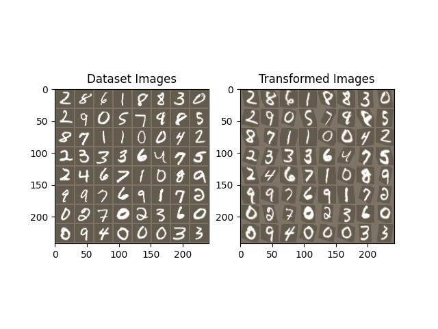
可视化 STN 结果#
现在,我们将检查我们学习到的视觉注意力机制的结果。
我们定义了一个小型辅助函数来可视化训练过程中的变换。
def convert_image_np(inp):
    """Convert a Tensor to numpy image."""
    inp = inp.numpy().transpose((1, 2, 0))
    mean = np.array([0.485, 0.456, 0.406])
    std = np.array([0.229, 0.224, 0.225])
    inp = std * inp + mean
    inp = np.clip(inp, 0, 1)
    return inp

# We want to visualize the output of the spatial transformers layer
# after the training, we visualize a batch of input images and
# the corresponding transformed batch using STN.


def visualize_stn():
    with torch.no_grad():
        # Get a batch of training data
        data = next(iter(test_loader))[0].to(device)

        input_tensor = data.cpu()
        transformed_input_tensor = model.stn(data).cpu()

        in_grid = convert_image_np(
            torchvision.utils.make_grid(input_tensor))

        out_grid = convert_image_np(
            torchvision.utils.make_grid(transformed_input_tensor))

        # Plot the results side-by-side
        f, axarr = plt.subplots(1, 2)
        axarr[0].imshow(in_grid)
        axarr[0].set_title('Dataset Images')

        axarr[1].imshow(out_grid)
        axarr[1].set_title('Transformed Images')

for epoch in range(1, 20 + 1):
    train(epoch)
    test()

# Visualize the STN transformation on some input batch
visualize_stn()

plt.ioff()
plt.show()
/usr/local/lib/python3.10/dist-packages/torch/nn/functional.py:5167: UserWarning:

Default grid_sample and affine_grid behavior has changed to align_corners=False since 1.3.0. Please specify align_corners=True if the old behavior is desired. See the documentation of grid_sample for details.

/usr/local/lib/python3.10/dist-packages/torch/nn/functional.py:5100: UserWarning:

Default grid_sample and affine_grid behavior has changed to align_corners=False since 1.3.0. Please specify align_corners=True if the old behavior is desired. See the documentation of grid_sample for details.

Train Epoch: 1 [0/60000 (0%)]   Loss: 2.321845
Train Epoch: 1 [32000/60000 (53%)]      Loss: 0.739860
/usr/local/lib/python3.10/dist-packages/torch/nn/_reduction.py:51: UserWarning:

size_average and reduce args will be deprecated, please use reduction='sum' instead.


Test set: Average loss: 0.2149, Accuracy: 9381/10000 (94%)

Train Epoch: 2 [0/60000 (0%)]   Loss: 0.310411
Train Epoch: 2 [32000/60000 (53%)]      Loss: 0.443614

Test set: Average loss: 0.1403, Accuracy: 9581/10000 (96%)

Train Epoch: 3 [0/60000 (0%)]   Loss: 0.184066
Train Epoch: 3 [32000/60000 (53%)]      Loss: 0.237139

Test set: Average loss: 0.0851, Accuracy: 9721/10000 (97%)

Train Epoch: 4 [0/60000 (0%)]   Loss: 0.235744
Train Epoch: 4 [32000/60000 (53%)]      Loss: 0.374082

Test set: Average loss: 0.0717, Accuracy: 9783/10000 (98%)

Train Epoch: 5 [0/60000 (0%)]   Loss: 0.209939
Train Epoch: 5 [32000/60000 (53%)]      Loss: 0.106230

Test set: Average loss: 0.0677, Accuracy: 9797/10000 (98%)

Train Epoch: 6 [0/60000 (0%)]   Loss: 0.210056
Train Epoch: 6 [32000/60000 (53%)]      Loss: 0.252697

Test set: Average loss: 0.0668, Accuracy: 9783/10000 (98%)

Train Epoch: 7 [0/60000 (0%)]   Loss: 0.123260
Train Epoch: 7 [32000/60000 (53%)]      Loss: 0.127563

Test set: Average loss: 0.0553, Accuracy: 9835/10000 (98%)

Train Epoch: 8 [0/60000 (0%)]   Loss: 0.108394
Train Epoch: 8 [32000/60000 (53%)]      Loss: 0.029457

Test set: Average loss: 0.0483, Accuracy: 9840/10000 (98%)

Train Epoch: 9 [0/60000 (0%)]   Loss: 0.176748
Train Epoch: 9 [32000/60000 (53%)]      Loss: 0.127248

Test set: Average loss: 0.1173, Accuracy: 9636/10000 (96%)

Train Epoch: 10 [0/60000 (0%)]  Loss: 0.243940
Train Epoch: 10 [32000/60000 (53%)]     Loss: 0.156468

Test set: Average loss: 0.2388, Accuracy: 9345/10000 (93%)

Train Epoch: 11 [0/60000 (0%)]  Loss: 0.378354
Train Epoch: 11 [32000/60000 (53%)]     Loss: 0.059640

Test set: Average loss: 0.0448, Accuracy: 9862/10000 (99%)

Train Epoch: 12 [0/60000 (0%)]  Loss: 0.129616
Train Epoch: 12 [32000/60000 (53%)]     Loss: 0.052506

Test set: Average loss: 0.0436, Accuracy: 9868/10000 (99%)

Train Epoch: 13 [0/60000 (0%)]  Loss: 0.045932
Train Epoch: 13 [32000/60000 (53%)]     Loss: 0.079384

Test set: Average loss: 0.0446, Accuracy: 9858/10000 (99%)

Train Epoch: 14 [0/60000 (0%)]  Loss: 0.031097
Train Epoch: 14 [32000/60000 (53%)]     Loss: 0.106284

Test set: Average loss: 0.0422, Accuracy: 9874/10000 (99%)

Train Epoch: 15 [0/60000 (0%)]  Loss: 0.133345
Train Epoch: 15 [32000/60000 (53%)]     Loss: 0.106248

Test set: Average loss: 0.0414, Accuracy: 9873/10000 (99%)

Train Epoch: 16 [0/60000 (0%)]  Loss: 0.044279
Train Epoch: 16 [32000/60000 (53%)]     Loss: 0.046603

Test set: Average loss: 0.0626, Accuracy: 9806/10000 (98%)

Train Epoch: 17 [0/60000 (0%)]  Loss: 0.157027
Train Epoch: 17 [32000/60000 (53%)]     Loss: 0.127502

Test set: Average loss: 0.0497, Accuracy: 9851/10000 (99%)

Train Epoch: 18 [0/60000 (0%)]  Loss: 0.041967
Train Epoch: 18 [32000/60000 (53%)]     Loss: 0.137598

Test set: Average loss: 0.0397, Accuracy: 9887/10000 (99%)

Train Epoch: 19 [0/60000 (0%)]  Loss: 0.115559
Train Epoch: 19 [32000/60000 (53%)]     Loss: 0.034766

Test set: Average loss: 0.0362, Accuracy: 9894/10000 (99%)

Train Epoch: 20 [0/60000 (0%)]  Loss: 0.078510
Train Epoch: 20 [32000/60000 (53%)]     Loss: 0.096980

Test set: Average loss: 0.0715, Accuracy: 9794/10000 (98%)
脚本总运行时间: (1 分钟 36.699 秒)
