


注意
跳转到末尾 下载完整的示例代码。
强化学习(DQN)教程#
创建于:2017年3月24日 | 最后更新:2025年6月16日 | 最后验证:2024年11月05日
本教程将展示如何使用 PyTorch 在 Gymnasium 的 CartPole-v1 任务上训练一个深度 Q-learning (DQN) 智能体。
你可能还会发现阅读原始的 深度 Q-learning (DQN) 论文很有帮助
任务
智能体需要在两个动作之间做出选择——向左或向右移动推车——以便连接到推车上的杆保持直立。你可以在 Gymnasium 的网站上找到关于该环境和其他更具挑战性环境的更多信息:Gymnasium 的网站。

CartPole#
当智能体观察到环境的当前状态并选择一个动作时,环境会转换到一个新状态,并返回一个奖励,该奖励指示动作的结果。在此任务中,每个增量时间步的奖励为 +1,如果杆倾斜过度或推车移出中心超过 2.4 个单位,环境将终止。这意味着表现更好的场景将运行更长时间,累积更高的回报。
CartPole 任务的设计使得智能体的输入是 4 个表示环境状态(位置、速度等)的实值。我们不经过任何缩放就采用这 4 个输入,并将它们通过一个小型的全连接网络,该网络有两个输出,分别对应两个动作。该网络经过训练,可以根据输入状态预测每个动作的预期值。然后选择具有最高预期值的动作。
包
首先,让我们导入所需的包。首先,我们需要 gymnasium 来处理环境,可以使用 pip 安装。这是原始 OpenAI Gym 项目的一个分支,自 Gym v0.19 起由同一团队维护。如果你在 Google Colab 中运行此代码,请执行
%%bash
pip3 install gymnasium[classic_control]
我们还将使用 PyTorch 的以下模块:
神经网络 (
torch.nn)优化 (
torch.optim)自动微分 (
torch.autograd)
import gymnasium as gym
import math
import random
import matplotlib
import matplotlib.pyplot as plt
from collections import namedtuple, deque
from itertools import count

import torch
import torch.nn as nn
import torch.optim as optim
import torch.nn.functional as F

env = gym.make("CartPole-v1")

# set up matplotlib
is_ipython = 'inline' in matplotlib.get_backend()
if is_ipython:
    from IPython import display

plt.ion()

# if GPU is to be used
device = torch.device(
    "cuda" if torch.cuda.is_available() else
    "mps" if torch.backends.mps.is_available() else
    "cpu"
)


# To ensure reproducibility during training, you can fix the random seeds
# by uncommenting the lines below. This makes the results consistent across
# runs, which is helpful for debugging or comparing different approaches.
#
# That said, allowing randomness can be beneficial in practice, as it lets
# the model explore different training trajectories.


# seed = 42
# random.seed(seed)
# torch.manual_seed(seed)
# env.reset(seed=seed)
# env.action_space.seed(seed)
# env.observation_space.seed(seed)
# if torch.cuda.is_available():
#     torch.cuda.manual_seed(seed)
Gym has been unmaintained since 2022 and does not support NumPy 2.0 amongst other critical functionality.
Please upgrade to Gymnasium, the maintained drop-in replacement of Gym, or contact the authors of your software and request that they upgrade.
Users of this version of Gym should be able to simply replace 'import gym' with 'import gymnasium as gym' in the vast majority of cases.
See the migration guide at https://gymnasium.org.cn/introduction/migration_guide/ for additional information.
经验回放#
我们将使用经验回放内存来训练我们的 DQN。它存储智能体观察到的转换,允许我们稍后重用这些数据。通过随机采样,构建批次的转换是去相关的。研究表明,这极大地稳定并改善了 DQN 的训练过程。
为此,我们需要两个类:
Transition- 一个命名元组,表示环境中的单个转换。它本质上是将(状态,动作)对映射到它们的(下一个状态,奖励)结果,其中状态是屏幕差异图像,如下文所述。ReplayMemory- 一个具有固定大小的循环缓冲区,用于存储最近观察到的转换。它还实现了一个.sample()方法,用于为训练选择随机批次的转换。
Transition = namedtuple('Transition',
                        ('state', 'action', 'next_state', 'reward'))


class ReplayMemory(object):

    def __init__(self, capacity):
        self.memory = deque([], maxlen=capacity)

    def push(self, *args):
        """Save a transition"""
        self.memory.append(Transition(*args))

    def sample(self, batch_size):
        return random.sample(self.memory, batch_size)

    def __len__(self):
        return len(self.memory)
现在,让我们定义我们的模型。但首先,让我们快速回顾一下 DQN 是什么。
DQN 算法#
我们的环境是确定性的,因此此处介绍的所有方程也以确定性的方式表述,以简化说明。在强化学习文献中,它们还包含对环境中随机转换的期望。
我们的目标是训练一个策略,该策略试图最大化折扣累积奖励 \(R_{t_0} = \sum_{t=t_0}^{\infty} \gamma^{t - t_0} r_t\),其中 \(R_{t_0}\) 也被称为回报。折扣因子 \(\gamma\) 必须是介于 \(0\) 和 \(1\) 之间的常数,以确保和收敛。较低的 \(\gamma\) 值使得未来不确定的奖励对我们的智能体的重要性不如它相当确定地能够获得的近期奖励。它还鼓励智能体比在未来时间上遥远的等效奖励更早地获得奖励。
Q-learning 的主要思想是,如果我们有一个函数 \(Q^*: State \times Action \rightarrow \mathbb{R}\),它可以告诉我们在给定状态下采取某个动作后,我们的回报将是多少,那么我们就可以很容易地构建一个最大化我们奖励的策略。
然而,我们并非全知世界,因此我们无法访问 \(Q^*\)。但是,由于神经网络是万能函数逼近器,我们可以简单地创建一个神经网络并训练它来逼近 \(Q^*\)。
对于我们的训练更新规则,我们将使用一个事实:任何 \(Q\) 函数对于某个策略都服从贝尔曼方程:
等式两边的差值称为时序差分误差,\(\delta\):
为了最小化这个误差,我们将使用 Huber 损失。当误差很小时,Huber 损失类似于均方误差,而当误差很大时,它类似于平均绝对误差——这使得它在 Q 估计非常嘈杂时对异常值更具鲁棒性。我们对从经验回放中采样的转换批次 \(B\) 计算此损失:
Q 网络#
我们的模型将是一个前馈神经网络,它接收当前屏幕帧和前一帧屏幕帧之间的差值作为输入。它有两个输出,分别表示 \(Q(s, \mathrm{left})\) 和 \(Q(s, \mathrm{right})\)(其中 \(s\) 是输入到网络的输入)。实际上,网络试图预测给定当前输入时采取每个动作的预期回报。
class DQN(nn.Module):

    def __init__(self, n_observations, n_actions):
        super(DQN, self).__init__()
        self.layer1 = nn.Linear(n_observations, 128)
        self.layer2 = nn.Linear(128, 128)
        self.layer3 = nn.Linear(128, n_actions)

    # Called with either one element to determine next action, or a batch
    # during optimization. Returns tensor([[left0exp,right0exp]...]).
    def forward(self, x):
        x = F.relu(self.layer1(x))
        x = F.relu(self.layer2(x))
        return self.layer3(x)
训练#
超参数和实用工具#
此单元格实例化我们的模型及其优化器,并定义了一些实用工具。
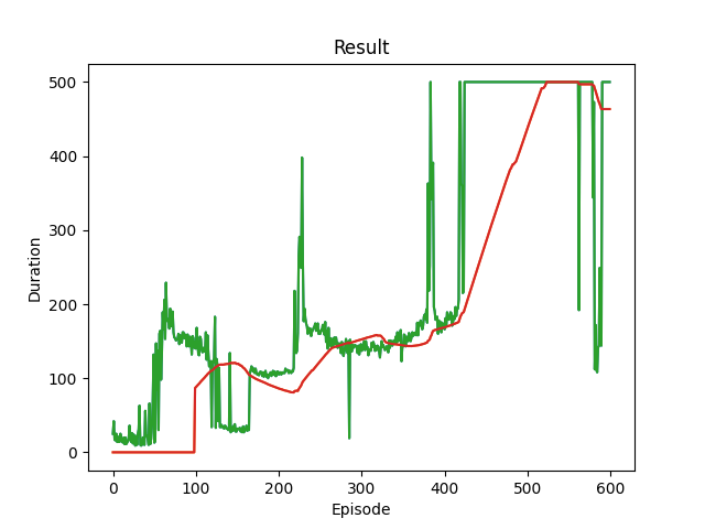
select_action- 将根据 epsilon 贪婪策略选择一个动作。简单来说,我们会偶尔使用我们的模型来选择动作,而有时我们会随机均匀采样一个动作。选择随机动作的概率将从EPS_START开始,并呈指数衰减到EPS_END。EPS_DECAY控制衰减速率。plot_durations- 一个辅助函数,用于绘制回合的持续时间,以及过去 100 回合的平均值(官方评估中使用的度量)。图表将显示在包含主训练循环的单元格下方,并在每个回合后更新。
# BATCH_SIZE is the number of transitions sampled from the replay buffer
# GAMMA is the discount factor as mentioned in the previous section
# EPS_START is the starting value of epsilon
# EPS_END is the final value of epsilon
# EPS_DECAY controls the rate of exponential decay of epsilon, higher means a slower decay
# TAU is the update rate of the target network
# LR is the learning rate of the ``AdamW`` optimizer

BATCH_SIZE = 128
GAMMA = 0.99
EPS_START = 0.9
EPS_END = 0.01
EPS_DECAY = 2500
TAU = 0.005
LR = 3e-4


# Get number of actions from gym action space
n_actions = env.action_space.n
# Get the number of state observations
state, info = env.reset()
n_observations = len(state)

policy_net = DQN(n_observations, n_actions).to(device)
target_net = DQN(n_observations, n_actions).to(device)
target_net.load_state_dict(policy_net.state_dict())

optimizer = optim.AdamW(policy_net.parameters(), lr=LR, amsgrad=True)
memory = ReplayMemory(10000)


steps_done = 0


def select_action(state):
    global steps_done
    sample = random.random()
    eps_threshold = EPS_END + (EPS_START - EPS_END) * \
        math.exp(-1. * steps_done / EPS_DECAY)
    steps_done += 1
    if sample > eps_threshold:
        with torch.no_grad():
            # t.max(1) will return the largest column value of each row.
            # second column on max result is index of where max element was
            # found, so we pick action with the larger expected reward.
            return policy_net(state).max(1).indices.view(1, 1)
    else:
        return torch.tensor([[env.action_space.sample()]], device=device, dtype=torch.long)


episode_durations = []


def plot_durations(show_result=False):
    plt.figure(1)
    durations_t = torch.tensor(episode_durations, dtype=torch.float)
    if show_result:
        plt.title('Result')
    else:
        plt.clf()
        plt.title('Training...')
    plt.xlabel('Episode')
    plt.ylabel('Duration')
    plt.plot(durations_t.numpy())
    # Take 100 episode averages and plot them too
    if len(durations_t) >= 100:
        means = durations_t.unfold(0, 100, 1).mean(1).view(-1)
        means = torch.cat((torch.zeros(99), means))
        plt.plot(means.numpy())

    plt.pause(0.001)  # pause a bit so that plots are updated
    if is_ipython:
        if not show_result:
            display.display(plt.gcf())
            display.clear_output(wait=True)
        else:
            display.display(plt.gcf())
训练循环#
最后,这是训练我们模型的代码。
在这里,你可以找到一个 optimize_model 函数,它执行单步优化。它首先采样一个批次,将所有张量连接成一个张量,计算 \(Q(s_t, a_t)\) 和 \(V(s_{t+1}) = \max_a Q(s_{t+1}, a)\),并将它们组合成我们的损失。根据定义,如果 \(s\) 是终止状态,我们将 \(V(s) = 0\)。我们还使用目标网络来计算 \(V(s_{t+1})\) 以增加稳定性。目标网络在每一步都使用由超参数 TAU 控制的软更新进行更新,TAU 之前已定义。
def optimize_model():
    if len(memory) < BATCH_SIZE:
        return
    transitions = memory.sample(BATCH_SIZE)
    # Transpose the batch (see https://stackoverflow.com/a/19343/3343043 for
    # detailed explanation). This converts batch-array of Transitions
    # to Transition of batch-arrays.
    batch = Transition(*zip(*transitions))

    # Compute a mask of non-final states and concatenate the batch elements
    # (a final state would've been the one after which simulation ended)
    non_final_mask = torch.tensor(tuple(map(lambda s: s is not None,
                                          batch.next_state)), device=device, dtype=torch.bool)
    non_final_next_states = torch.cat([s for s in batch.next_state
                                                if s is not None])
    state_batch = torch.cat(batch.state)
    action_batch = torch.cat(batch.action)
    reward_batch = torch.cat(batch.reward)

    # Compute Q(s_t, a) - the model computes Q(s_t), then we select the
    # columns of actions taken. These are the actions which would've been taken
    # for each batch state according to policy_net
    state_action_values = policy_net(state_batch).gather(1, action_batch)

    # Compute V(s_{t+1}) for all next states.
    # Expected values of actions for non_final_next_states are computed based
    # on the "older" target_net; selecting their best reward with max(1).values
    # This is merged based on the mask, such that we'll have either the expected
    # state value or 0 in case the state was final.
    next_state_values = torch.zeros(BATCH_SIZE, device=device)
    with torch.no_grad():
        next_state_values[non_final_mask] = target_net(non_final_next_states).max(1).values
    # Compute the expected Q values
    expected_state_action_values = (next_state_values * GAMMA) + reward_batch

    # Compute Huber loss
    criterion = nn.SmoothL1Loss()
    loss = criterion(state_action_values, expected_state_action_values.unsqueeze(1))

    # Optimize the model
    optimizer.zero_grad()
    loss.backward()
    # In-place gradient clipping
    torch.nn.utils.clip_grad_value_(policy_net.parameters(), 100)
    optimizer.step()
下面是主训练循环。开始时,我们重置环境并获取初始 state 张量。然后,我们采样一个动作,执行它,观察下一个状态和奖励(始终为 1),并对我们的模型进行一次优化。当回合结束时(我们的模型失败),我们重新启动循环。
下面,如果可用 GPU,num_episodes 设置为 600;否则,安排 50 个回合,以免训练时间过长。然而,50 个回合不足以在 CartPole 上观察到良好性能。你应该会看到模型在 600 个训练回合内持续达到 500 步。训练 RL 智能体可能是一个不确定的过程,因此如果未观察到收敛,重新开始训练可以产生更好的结果。
if torch.cuda.is_available() or torch.backends.mps.is_available():
    num_episodes = 600
else:
    num_episodes = 50

for i_episode in range(num_episodes):
    # Initialize the environment and get its state
    state, info = env.reset()
    state = torch.tensor(state, dtype=torch.float32, device=device).unsqueeze(0)
    for t in count():
        action = select_action(state)
        observation, reward, terminated, truncated, _ = env.step(action.item())
        reward = torch.tensor([reward], device=device)
        done = terminated or truncated

        if terminated:
            next_state = None
        else:
            next_state = torch.tensor(observation, dtype=torch.float32, device=device).unsqueeze(0)

        # Store the transition in memory
        memory.push(state, action, next_state, reward)

        # Move to the next state
        state = next_state

        # Perform one step of the optimization (on the policy network)
        optimize_model()

        # Soft update of the target network's weights
        # θ′ ← τ θ + (1 −τ )θ′
        target_net_state_dict = target_net.state_dict()
        policy_net_state_dict = policy_net.state_dict()
        for key in policy_net_state_dict:
            target_net_state_dict[key] = policy_net_state_dict[key]*TAU + target_net_state_dict[key]*(1-TAU)
        target_net.load_state_dict(target_net_state_dict)

        if done:
            episode_durations.append(t + 1)
            plot_durations()
            break

print('Complete')
plot_durations(show_result=True)
plt.ioff()
plt.show()
/usr/local/lib/python3.10/dist-packages/gymnasium/utils/passive_env_checker.py:249: DeprecationWarning:

`np.bool8` is a deprecated alias for `np.bool_`.  (Deprecated NumPy 1.24)

Complete
这是说明总体结果数据流的图表。
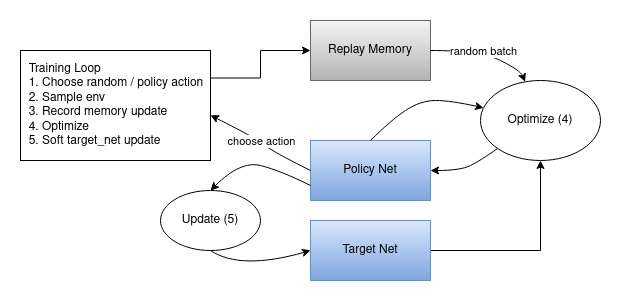
动作是随机选择的,或者基于策略选择的,从 gym 环境中获取下一步的样本。我们将结果记录在经验回放中,并在每次迭代时进行优化。优化从经验回放中随机抽取一个批次来训练新策略。用于计算预期 Q 值的“旧”目标网络也用于优化。其权重在每一步都会进行软更新。
脚本总运行时间: (6 分钟 48.617 秒)
