


使用 TensorBoard 可视化模型、数据和训练#
创建日期:2019 年 8 月 8 日 | 最后更新:2025 年 9 月 10 日 | 最后验证:2024 年 11 月 5 日
在 60 分钟快速教程 中,我们向您展示了如何加载数据,将其输入到我们定义为 nn.Module 子类的模型中,在训练数据上训练此模型,并在测试数据上对其进行测试。为了查看正在发生的情况,我们在模型训练时打印出一些统计信息,以了解训练是否在进展。但是,我们可以做得更好:PyTorch 与 TensorBoard 集成,TensorBoard 是一个用于可视化神经网络训练运行结果的工具。本教程将演示其部分功能,使用 Fashion-MNIST 数据集,该数据集可以使用 torchvision.datasets 加载到 PyTorch 中。
在本教程中,我们将学习如何
读取数据并进行适当的转换(与之前的教程几乎相同)。
设置 TensorBoard。
写入 TensorBoard。
使用 TensorBoard 检查模型架构。
使用 TensorBoard 以更少的代码创建上一个教程中创建的可视化的交互式版本
具体来说,在第 5 点,我们将看到
几种检查训练数据的方法
如何跟踪模型的训练过程中的性能
如何评估模型训练完成后的性能。
我们将从与 CIFAR-10 教程 相似的样板代码开始
# imports
import matplotlib.pyplot as plt
import numpy as np

import torch
import torchvision
import torchvision.transforms as transforms

import torch.nn as nn
import torch.nn.functional as F
import torch.optim as optim

# transforms
transform = transforms.Compose(
    [transforms.ToTensor(),
    transforms.Normalize((0.5,), (0.5,))])

# datasets
trainset = torchvision.datasets.FashionMNIST('./data',
    download=True,
    train=True,
    transform=transform)
testset = torchvision.datasets.FashionMNIST('./data',
    download=True,
    train=False,
    transform=transform)

# dataloaders
trainloader = torch.utils.data.DataLoader(trainset, batch_size=4, shuffle=True)

testloader = torch.utils.data.DataLoader(testset, batch_size=4, shuffle=False)

# constant for classes
classes = ('T-shirt/top', 'Trouser', 'Pullover', 'Dress', 'Coat',
        'Sandal', 'Shirt', 'Sneaker', 'Bag', 'Ankle Boot')

# helper function to show an image
# (used in the `plot_classes_preds` function below)
def matplotlib_imshow(img, one_channel=False):
    if one_channel:
        img = img.mean(dim=0)
    img = img / 2 + 0.5     # unnormalize
    npimg = img.numpy()
    if one_channel:
        plt.imshow(npimg, cmap="Greys")
    else:
        plt.imshow(np.transpose(npimg, (1, 2, 0)))
我们将定义一个与该教程类似的相似模型架构,仅进行少量修改,以适应图像现在是一个通道而非三个通道,以及 28x28 而非 32x32 的事实
class Net(nn.Module):
    def __init__(self):
        super(Net, self).__init__()
        self.conv1 = nn.Conv2d(1, 6, 5)
        self.pool = nn.MaxPool2d(2, 2)
        self.conv2 = nn.Conv2d(6, 16, 5)
        self.fc1 = nn.Linear(16 * 4 * 4, 120)
        self.fc2 = nn.Linear(120, 84)
        self.fc3 = nn.Linear(84, 10)

    def forward(self, x):
        x = self.pool(F.relu(self.conv1(x)))
        x = self.pool(F.relu(self.conv2(x)))
        x = x.view(-1, 16 * 4 * 4)
        x = F.relu(self.fc1(x))
        x = F.relu(self.fc2(x))
        x = self.fc3(x)
        return x


net = Net()
我们将定义之前相同的 optimizer 和 criterion
criterion = nn.CrossEntropyLoss()
optimizer = optim.SGD(net.parameters(), lr=0.001, momentum=0.9)
1. TensorBoard 设置#
现在我们将设置 TensorBoard,从 torch.utils 导入 tensorboard,并定义一个 SummaryWriter,这是我们向 TensorBoard 写入信息的主要对象。
from torch.utils.tensorboard import SummaryWriter

# default `log_dir` is "runs" - we'll be more specific here
writer = SummaryWriter('runs/fashion_mnist_experiment_1')
请注意,仅这一行就会创建一个 runs/fashion_mnist_experiment_1 文件夹。
2. 写入 TensorBoard#
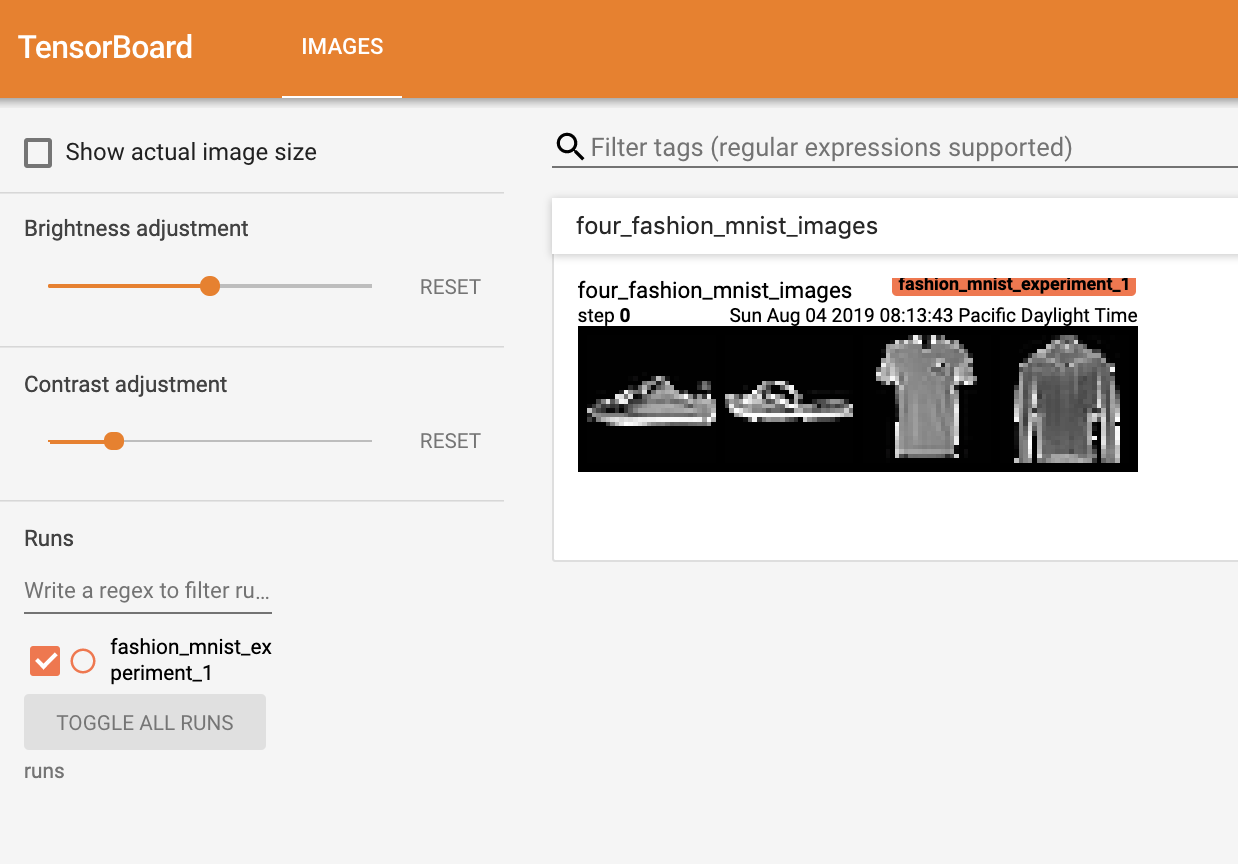
现在让我们使用 make_grid 将一个图像写入我们的 TensorBoard - 特别是一个网格。
# get some random training images
dataiter = iter(trainloader)
images, labels = next(dataiter)

# create grid of images
img_grid = torchvision.utils.make_grid(images)

# show images
matplotlib_imshow(img_grid, one_channel=True)

# write to tensorboard
writer.add_image('four_fashion_mnist_images', img_grid)
现在从命令行运行
PYTHONWARNINGS="ignore:pkg_resources is deprecated as an API:UserWarning" tensorboard --logdir=runs
然后导航到 https://:6006 应该会显示以下内容。
现在您知道如何使用 TensorBoard 了!但是,这个例子可以在 Jupyter Notebook 中完成 — TensorBoard 真正擅长的是创建交互式可视化。我们将在下一个教程中介绍其中一个,并在本教程结束时介绍更多。
3. 使用 TensorBoard 检查模型#
TensorBoard 的优势之一是其可视化复杂模型结构的能力。让我们可视化我们构建的模型。
writer.add_graph(net, images)
writer.close()
现在刷新 TensorBoard 后,您应该会看到一个“Graphs”选项卡,看起来像这样
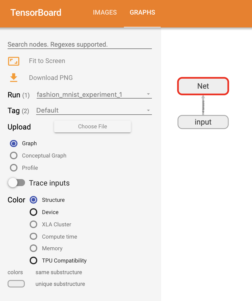
请双击“Net”以查看其展开,看到构成模型的各个操作的详细视图。
TensorBoard 有一个非常有用的功能,可以可视化高维数据,如图像数据在低维空间中的表示;我们将在下一节介绍。
4. 为 TensorBoard 添加“Projector”#
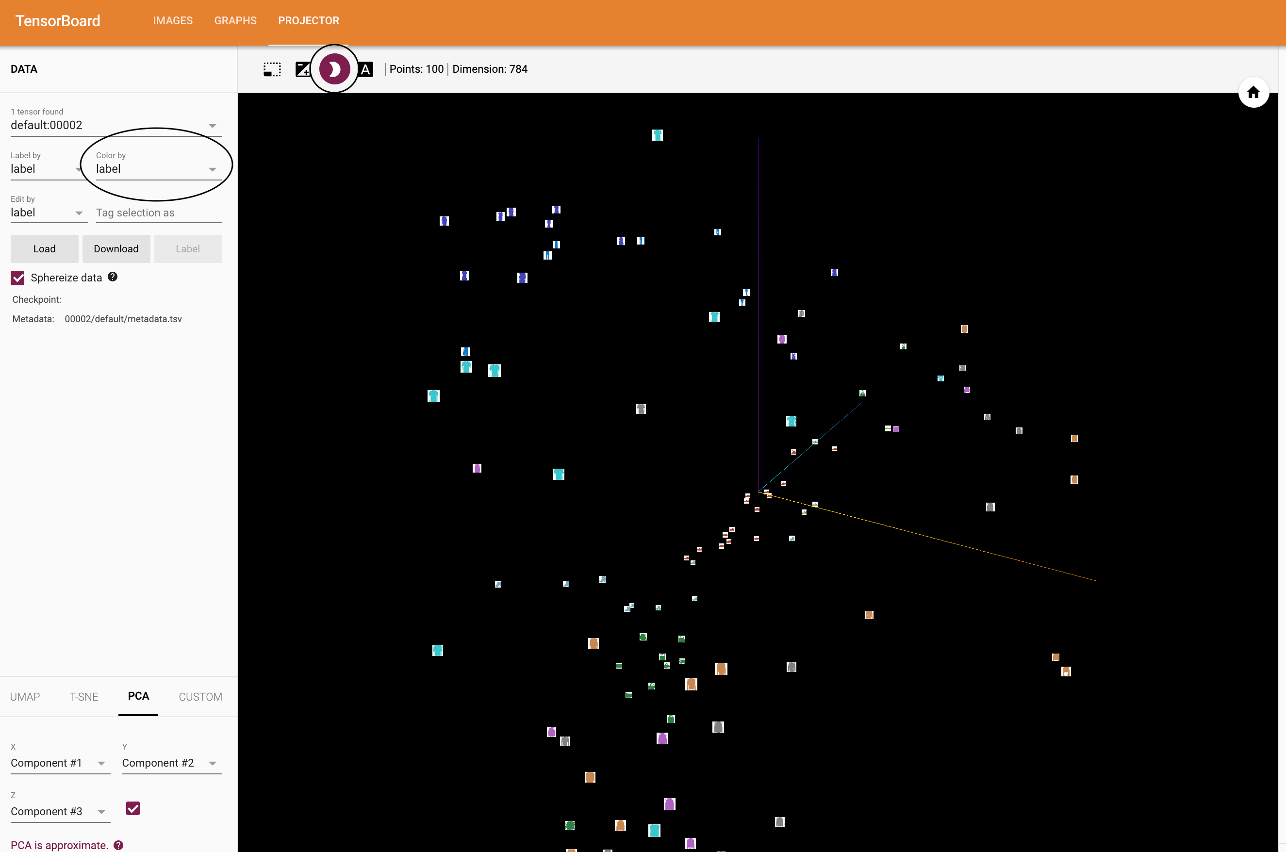
我们可以通过 add_embedding 方法可视化高维数据的低维表示
# helper function
def select_n_random(data, labels, n=100):
    '''
    Selects n random datapoints and their corresponding labels from a dataset
    '''
    assert len(data) == len(labels)

    perm = torch.randperm(len(data))
    return data[perm][:n], labels[perm][:n]

# select random images and their target indices
images, labels = select_n_random(trainset.data, trainset.targets)

# get the class labels for each image
class_labels = [classes[lab] for lab in labels]

# log embeddings
features = images.view(-1, 28 * 28)
writer.add_embedding(features,
                    metadata=class_labels,
                    label_img=images.unsqueeze(1))
writer.close()
现在在 TensorBoard 的“Projector”选项卡中,您可以看到这 100 张图像 — 每张图像都有 784 维 — 被投影到三维空间中。此外,这是交互式的:您可以单击并拖动以旋转三维投影。最后,有几个技巧可以使可视化更容易查看:选择左上角的“color: label”,以及启用“night mode”,这将使图像更容易看到,因为它们的背景是白色的
现在我们已经仔细检查了我们的数据,让我们展示 TensorBoard 如何使跟踪模型训练和评估更加清晰,从训练开始。
5. 使用 TensorBoard 跟踪模型训练#
在之前的示例中,我们只是每 2000 次迭代 *打印* 模型的运行损失。现在,我们将把运行损失记录到 TensorBoard,并通过 plot_classes_preds 函数提供模型预测的视图。
# helper functions

def images_to_probs(net, images):
    '''
    Generates predictions and corresponding probabilities from a trained
    network and a list of images
    '''
    output = net(images)
    # convert output probabilities to predicted class
    _, preds_tensor = torch.max(output, 1)
    preds = np.squeeze(preds_tensor.numpy())
    return preds, [F.softmax(el, dim=0)[i].item() for i, el in zip(preds, output)]


def plot_classes_preds(net, images, labels):
    '''
    Generates matplotlib Figure using a trained network, along with images
    and labels from a batch, that shows the network's top prediction along
    with its probability, alongside the actual label, coloring this
    information based on whether the prediction was correct or not.
    Uses the "images_to_probs" function.
    '''
    preds, probs = images_to_probs(net, images)
    # plot the images in the batch, along with predicted and true labels
    fig = plt.figure(figsize=(12, 48))
    for idx in np.arange(4):
        ax = fig.add_subplot(1, 4, idx+1, xticks=[], yticks=[])
        matplotlib_imshow(images[idx], one_channel=True)
        ax.set_title("{0}, {1:.1f}%\n(label: {2})".format(
            classes[preds[idx]],
            probs[idx] * 100.0,
            classes[labels[idx]]),
                    color=("green" if preds[idx]==labels[idx].item() else "red"))
    return fig
最后,让我们使用与先前教程相同的模型训练代码来训练模型,但每 1000 个批次将结果写入 TensorBoard,而不是打印到控制台;这是通过 add_scalar 函数实现的。
此外,在训练过程中,我们将生成一张图像,显示模型在批次中包含的四张图像上的预测与实际结果。
running_loss = 0.0
for epoch in range(1):  # loop over the dataset multiple times

    for i, data in enumerate(trainloader, 0):

        # get the inputs; data is a list of [inputs, labels]
        inputs, labels = data

        # zero the parameter gradients
        optimizer.zero_grad()

        # forward + backward + optimize
        outputs = net(inputs)
        loss = criterion(outputs, labels)
        loss.backward()
        optimizer.step()

        running_loss += loss.item()
        if i % 1000 == 999:    # every 1000 mini-batches...

            # ...log the running loss
            writer.add_scalar('training loss',
                            running_loss / 1000,
                            epoch * len(trainloader) + i)

            # ...log a Matplotlib Figure showing the model's predictions on a
            # random mini-batch
            writer.add_figure('predictions vs. actuals',
                            plot_classes_preds(net, inputs, labels),
                            global_step=epoch * len(trainloader) + i)
            running_loss = 0.0
print('Finished Training')
您现在可以查看 scalars 选项卡,查看在 15,000 次训练迭代中绘制的运行损失图
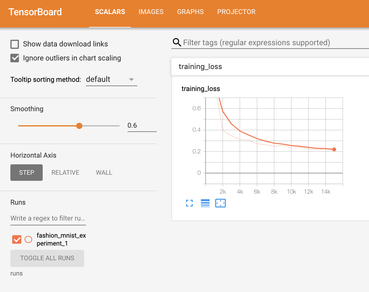
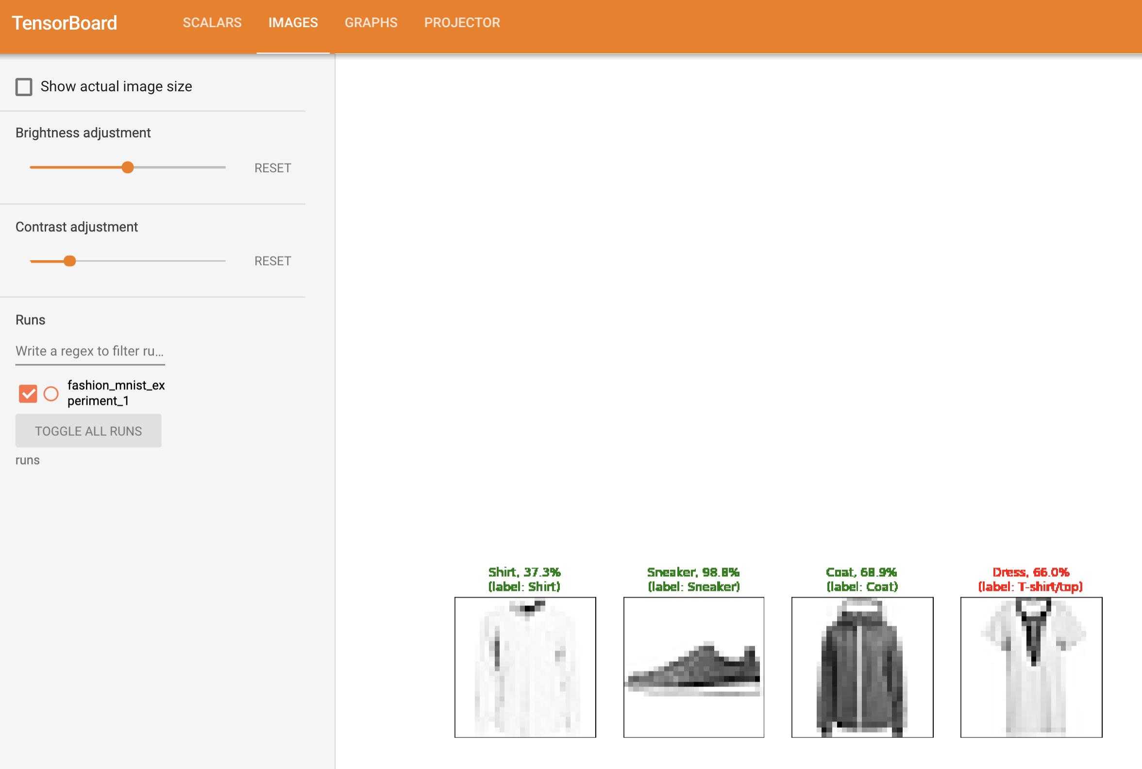
此外,我们可以查看模型在学习过程中对任意批次的预测。查看“Images”选项卡,并在“predictions vs. actuals”可视化下方滚动,可以看到这一点;这表明,例如,在仅 3000 次训练迭代后,模型已经能够区分视觉上不同的类,如衬衫、运动鞋和外套,尽管它不像在训练后期那样自信
在先前的教程中,我们查看了模型训练完成后的每个类别的准确率;在这里,我们将使用 TensorBoard 为每个类绘制精确率-召回率曲线(在此处有很好的解释 here)。
6. 评估训练好的模型#
# 1. gets the probability predictions in a test_size x num_classes Tensor
# 2. gets the preds in a test_size Tensor
# takes ~10 seconds to run
class_probs = []
class_label = []
with torch.no_grad():
    for data in testloader:
        images, labels = data
        output = net(images)
        class_probs_batch = [F.softmax(el, dim=0) for el in output]

        class_probs.append(class_probs_batch)
        class_label.append(labels)

test_probs = torch.cat([torch.stack(batch) for batch in class_probs])
test_label = torch.cat(class_label)

# helper function
def add_pr_curve_tensorboard(class_index, test_probs, test_label, global_step=0):
    '''
    Takes in a "class_index" from 0 to 9 and plots the corresponding
    precision-recall curve
    '''
    tensorboard_truth = test_label == class_index
    tensorboard_probs = test_probs[:, class_index]

    writer.add_pr_curve(classes[class_index],
                        tensorboard_truth,
                        tensorboard_probs,
                        global_step=global_step)
    writer.close()

# plot all the pr curves
for i in range(len(classes)):
    add_pr_curve_tensorboard(i, test_probs, test_label)
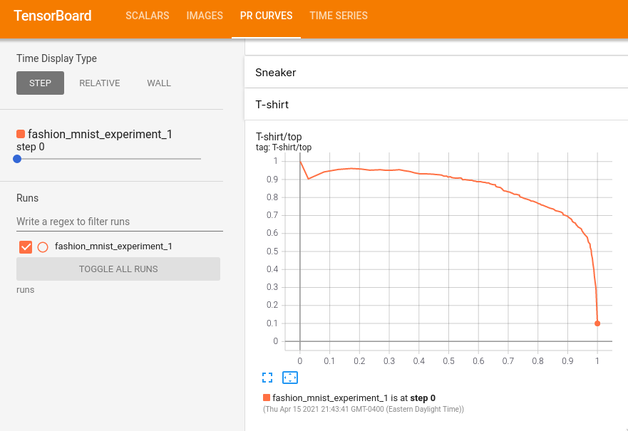
您现在将看到一个包含每个类别的精确率-召回率曲线的“PR Curves”选项卡。请随意探索;您会发现,在某些类别上,模型的“曲线下面积”接近 100%,而在其他类别上,这个面积较低
这就是 TensorBoard 和 PyTorch 与其集成的入门介绍。当然,您可以在 Jupyter Notebook 中完成 TensorBoard 的所有功能,但有了 TensorBoard,您将获得默认的交互式可视化。
