


注意
请 跳转到末尾 下载完整的示例代码。
训练分类器#
创建日期:2017 年 3 月 24 日 | 最后更新:2025 年 9 月 30 日 | 最后验证:未经验证
就是这样。您已经了解了如何定义神经网络、计算损失以及更新网络权重。
现在您可能会想,
数据呢?#
通常,当您需要处理图像、文本、音频或视频数据时,可以使用标准的 Python 包将数据加载到 NumPy 数组中。然后,您可以将此数组转换为 torch.*Tensor。
对于图像,Pillow、OpenCV 等包非常有用。
对于音频,scipy 和 librosa 等包非常有用。
对于文本,可以使用纯 Python 或基于 Cython 的加载,或者 NLTK 和 SpaCy。
特别是对于视觉领域,我们创建了一个名为 torchvision 的包,它提供了常见数据集(如 ImageNet、CIFAR10、MNIST 等)的数据加载器以及图像数据转换器,即 torchvision.datasets 和 torch.utils.data.DataLoader。
这提供了极大的便利,并避免了编写样板代码。
在本教程中,我们将使用 CIFAR10 数据集。它包含以下类别:“飞机”、“汽车”、“鸟”、“猫”、“鹿”、“狗”、“青蛙”、“马”、“船”、“卡车”。CIFAR-10 中的图像尺寸为 3x32x32,即 3 通道的彩色图像,尺寸为 32x32 像素。
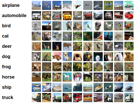
cifar10#
训练图像分类器#
我们将按顺序执行以下步骤:
使用
torchvision加载和归一化 CIFAR10 训练集和测试集。定义一个卷积神经网络。
定义一个损失函数。
在训练数据上训练网络。
在测试数据上测试网络。
1. 加载和归一化 CIFAR10#
使用 torchvision 加载 CIFAR10 非常简单。
import torch
import torchvision
import torchvision.transforms as transforms
torchvision 数据集的输出是 PILImage 图像,范围为 [0, 1]。我们将其转换为归一化范围 [-1, 1] 的 Tensor。
注意
如果您在 Windows 或 MacOS 上运行此教程,并遇到与多进程相关的 BrokenPipeError 或 RuntimeError,请尝试将 `torch.utils.data.DataLoader()` 的 `num_worker` 设置为 0。
transform = transforms.Compose(
    [transforms.ToTensor(),
     transforms.Normalize((0.5, 0.5, 0.5), (0.5, 0.5, 0.5))])

batch_size = 4

trainset = torchvision.datasets.CIFAR10(root='./data', train=True,
                                        download=True, transform=transform)
trainloader = torch.utils.data.DataLoader(trainset, batch_size=batch_size,
                                          shuffle=True, num_workers=2)

testset = torchvision.datasets.CIFAR10(root='./data', train=False,
                                       download=True, transform=transform)
testloader = torch.utils.data.DataLoader(testset, batch_size=batch_size,
                                         shuffle=False, num_workers=2)

classes = ('plane', 'car', 'bird', 'cat',
           'deer', 'dog', 'frog', 'horse', 'ship', 'truck')
  0%|          | 0.00/170M [00:00<?, ?B/s]
  0%|          | 328k/170M [00:00<00:53, 3.18MB/s]
  1%|          | 950k/170M [00:00<00:34, 4.85MB/s]
  1%|          | 1.70M/170M [00:00<00:28, 6.01MB/s]
  2%|▏         | 2.65M/170M [00:00<00:22, 7.30MB/s]
  2%|▏         | 3.80M/170M [00:00<00:19, 8.74MB/s]
  3%|▎         | 5.05M/170M [00:00<00:16, 9.96MB/s]
  4%|▎         | 6.23M/170M [00:00<00:15, 10.4MB/s]
  4%|▍         | 7.27M/170M [00:00<00:16, 9.98MB/s]
  5%|▍         | 8.29M/170M [00:00<00:16, 9.69MB/s]
  5%|▌         | 9.27M/170M [00:01<00:17, 9.33MB/s]
  6%|▌         | 10.2M/170M [00:01<00:17, 9.01MB/s]
  7%|▋         | 11.1M/170M [00:01<00:17, 8.94MB/s]
  7%|▋         | 12.1M/170M [00:01<00:17, 8.94MB/s]
  8%|▊         | 13.0M/170M [00:01<00:17, 8.95MB/s]
  8%|▊         | 14.0M/170M [00:01<00:17, 9.18MB/s]
  9%|▊         | 14.9M/170M [00:01<00:16, 9.18MB/s]
  9%|▉         | 15.9M/170M [00:01<00:17, 9.09MB/s]
 10%|▉         | 16.8M/170M [00:01<00:16, 9.09MB/s]
 10%|█         | 17.7M/170M [00:01<00:16, 9.10MB/s]
 11%|█         | 18.6M/170M [00:02<00:16, 9.05MB/s]
 11%|█▏        | 19.5M/170M [00:02<00:16, 9.03MB/s]
 12%|█▏        | 20.4M/170M [00:02<00:16, 9.04MB/s]
 13%|█▎        | 21.4M/170M [00:02<00:16, 8.99MB/s]
 13%|█▎        | 22.3M/170M [00:02<00:16, 8.84MB/s]
 14%|█▎        | 23.2M/170M [00:02<00:16, 8.78MB/s]
 14%|█▍        | 24.1M/170M [00:02<00:16, 8.66MB/s]
 15%|█▍        | 25.0M/170M [00:02<00:17, 8.28MB/s]
 15%|█▌        | 25.8M/170M [00:02<00:18, 7.94MB/s]
 16%|█▌        | 26.6M/170M [00:03<00:18, 7.66MB/s]
 16%|█▌        | 27.4M/170M [00:03<00:19, 7.49MB/s]
 17%|█▋        | 28.2M/170M [00:03<00:19, 7.32MB/s]
 17%|█▋        | 28.9M/170M [00:03<00:19, 7.20MB/s]
 17%|█▋        | 29.7M/170M [00:03<00:19, 7.08MB/s]
 18%|█▊        | 30.4M/170M [00:03<00:19, 7.01MB/s]
 18%|█▊        | 31.1M/170M [00:03<00:19, 6.99MB/s]
 19%|█▊        | 31.8M/170M [00:03<00:19, 6.98MB/s]
 19%|█▉        | 32.5M/170M [00:03<00:20, 6.90MB/s]
 20%|█▉        | 33.3M/170M [00:04<00:20, 6.80MB/s]
 20%|█▉        | 33.9M/170M [00:04<00:20, 6.71MB/s]
 20%|██        | 34.6M/170M [00:04<00:20, 6.65MB/s]
 21%|██        | 35.3M/170M [00:04<00:20, 6.61MB/s]
 21%|██        | 36.0M/170M [00:04<00:20, 6.58MB/s]
 22%|██▏       | 36.7M/170M [00:04<00:20, 6.55MB/s]
 22%|██▏       | 37.4M/170M [00:04<00:20, 6.54MB/s]
 22%|██▏       | 38.0M/170M [00:04<00:20, 6.51MB/s]
 23%|██▎       | 38.7M/170M [00:04<00:20, 6.47MB/s]
 23%|██▎       | 39.3M/170M [00:04<00:20, 6.40MB/s]
 23%|██▎       | 40.0M/170M [00:05<00:20, 6.27MB/s]
 24%|██▍       | 40.6M/170M [00:05<00:21, 6.16MB/s]
 24%|██▍       | 41.3M/170M [00:05<00:21, 6.09MB/s]
 25%|██▍       | 41.9M/170M [00:05<00:21, 6.11MB/s]
 25%|██▍       | 42.5M/170M [00:05<00:21, 6.09MB/s]
 25%|██▌       | 43.2M/170M [00:05<00:20, 6.13MB/s]
 26%|██▌       | 43.8M/170M [00:05<00:20, 6.12MB/s]
 26%|██▌       | 44.4M/170M [00:05<00:20, 6.14MB/s]
 26%|██▋       | 45.1M/170M [00:05<00:20, 6.16MB/s]
 27%|██▋       | 45.7M/170M [00:06<00:20, 6.23MB/s]
 27%|██▋       | 46.4M/170M [00:06<00:20, 6.19MB/s]
 28%|██▊       | 47.0M/170M [00:06<00:19, 6.19MB/s]
 28%|██▊       | 47.6M/170M [00:06<00:19, 6.29MB/s]
 28%|██▊       | 48.3M/170M [00:06<00:19, 6.33MB/s]
 29%|██▊       | 49.0M/170M [00:06<00:19, 6.39MB/s]
 29%|██▉       | 49.6M/170M [00:06<00:18, 6.36MB/s]
 29%|██▉       | 50.3M/170M [00:06<00:19, 6.25MB/s]
 30%|██▉       | 50.9M/170M [00:06<00:19, 6.09MB/s]
 30%|███       | 51.5M/170M [00:06<00:19, 5.98MB/s]
 31%|███       | 52.2M/170M [00:07<00:19, 5.93MB/s]
 31%|███       | 52.8M/170M [00:07<00:20, 5.82MB/s]
 31%|███▏      | 53.4M/170M [00:07<00:20, 5.72MB/s]
 32%|███▏      | 54.0M/170M [00:07<00:20, 5.57MB/s]
 32%|███▏      | 54.6M/170M [00:07<00:21, 5.47MB/s]
 32%|███▏      | 55.1M/170M [00:07<00:21, 5.35MB/s]
 33%|███▎      | 55.7M/170M [00:07<00:21, 5.26MB/s]
 33%|███▎      | 56.2M/170M [00:07<00:22, 5.19MB/s]
 33%|███▎      | 56.8M/170M [00:07<00:22, 5.16MB/s]
 34%|███▎      | 57.3M/170M [00:08<00:22, 5.14MB/s]
 34%|███▍      | 57.8M/170M [00:08<00:22, 5.05MB/s]
 34%|███▍      | 58.3M/170M [00:08<00:22, 5.09MB/s]
 35%|███▍      | 58.9M/170M [00:08<00:22, 5.06MB/s]
 35%|███▍      | 59.4M/170M [00:08<00:21, 5.07MB/s]
 35%|███▌      | 59.9M/170M [00:08<00:21, 5.09MB/s]
 35%|███▌      | 60.4M/170M [00:08<00:21, 5.08MB/s]
 36%|███▌      | 60.9M/170M [00:08<00:21, 5.07MB/s]
 36%|███▌      | 61.5M/170M [00:08<00:21, 5.07MB/s]
 36%|███▋      | 62.0M/170M [00:08<00:21, 5.09MB/s]
 37%|███▋      | 62.5M/170M [00:09<00:21, 5.10MB/s]
 37%|███▋      | 63.0M/170M [00:09<00:21, 5.11MB/s]
 37%|███▋      | 63.6M/170M [00:09<00:21, 5.08MB/s]
 38%|███▊      | 64.1M/170M [00:09<00:20, 5.10MB/s]
 38%|███▊      | 64.6M/170M [00:09<00:20, 5.10MB/s]
 38%|███▊      | 65.1M/170M [00:09<00:20, 5.08MB/s]
 39%|███▊      | 65.7M/170M [00:09<00:20, 5.09MB/s]
 39%|███▉      | 66.2M/170M [00:09<00:20, 5.11MB/s]
 39%|███▉      | 66.7M/170M [00:09<00:20, 5.06MB/s]
 39%|███▉      | 67.2M/170M [00:10<00:20, 5.09MB/s]
 40%|███▉      | 67.8M/170M [00:10<00:20, 5.10MB/s]
 40%|████      | 68.3M/170M [00:10<00:20, 5.08MB/s]
 40%|████      | 68.8M/170M [00:10<00:19, 5.09MB/s]
 41%|████      | 69.3M/170M [00:10<00:19, 5.07MB/s]
 41%|████      | 69.9M/170M [00:10<00:19, 5.07MB/s]
 41%|████▏     | 70.4M/170M [00:10<00:19, 5.08MB/s]
 42%|████▏     | 70.9M/170M [00:10<00:19, 5.10MB/s]
 42%|████▏     | 71.4M/170M [00:10<00:19, 5.07MB/s]
 42%|████▏     | 72.0M/170M [00:10<00:19, 5.07MB/s]
 43%|████▎     | 72.5M/170M [00:11<00:19, 5.00MB/s]
 43%|████▎     | 73.0M/170M [00:11<00:19, 4.98MB/s]
 43%|████▎     | 73.5M/170M [00:11<00:19, 4.95MB/s]
 43%|████▎     | 74.1M/170M [00:11<00:19, 4.89MB/s]
 44%|████▎     | 74.5M/170M [00:11<00:19, 4.87MB/s]
 44%|████▍     | 75.1M/170M [00:11<00:19, 4.88MB/s]
 44%|████▍     | 75.6M/170M [00:11<00:19, 4.89MB/s]
 45%|████▍     | 76.1M/170M [00:11<00:19, 4.92MB/s]
 45%|████▍     | 76.6M/170M [00:11<00:19, 4.91MB/s]
 45%|████▌     | 77.1M/170M [00:12<00:18, 4.93MB/s]
 46%|████▌     | 77.7M/170M [00:12<00:18, 4.93MB/s]
 46%|████▌     | 78.2M/170M [00:12<00:19, 4.78MB/s]
 46%|████▌     | 78.7M/170M [00:12<00:18, 4.95MB/s]
 46%|████▋     | 79.3M/170M [00:12<00:18, 5.02MB/s]
 47%|████▋     | 79.8M/170M [00:12<00:18, 5.04MB/s]
 47%|████▋     | 80.3M/170M [00:12<00:17, 5.02MB/s]
 47%|████▋     | 80.8M/170M [00:12<00:17, 5.01MB/s]
 48%|████▊     | 81.4M/170M [00:12<00:17, 4.99MB/s]
 48%|████▊     | 81.9M/170M [00:12<00:17, 5.03MB/s]
 48%|████▊     | 82.4M/170M [00:13<00:17, 4.93MB/s]
 49%|████▊     | 82.9M/170M [00:13<00:17, 4.96MB/s]
 49%|████▉     | 83.5M/170M [00:13<00:17, 4.95MB/s]
 49%|████▉     | 84.0M/170M [00:13<00:17, 4.97MB/s]
 50%|████▉     | 84.5M/170M [00:13<00:17, 4.84MB/s]
 50%|████▉     | 85.0M/170M [00:13<00:17, 4.78MB/s]
 50%|█████     | 85.5M/170M [00:13<00:18, 4.70MB/s]
 50%|█████     | 86.0M/170M [00:13<00:18, 4.67MB/s]
 51%|█████     | 86.5M/170M [00:13<00:18, 4.64MB/s]
 51%|█████     | 87.0M/170M [00:14<00:18, 4.63MB/s]
 51%|█████▏    | 87.5M/170M [00:14<00:18, 4.56MB/s]
 52%|█████▏    | 87.9M/170M [00:14<00:18, 4.54MB/s]
 52%|█████▏    | 88.4M/170M [00:14<00:18, 4.54MB/s]
 52%|█████▏    | 88.8M/170M [00:14<00:18, 4.49MB/s]
 52%|█████▏    | 89.3M/170M [00:14<00:18, 4.49MB/s]
 53%|█████▎    | 89.8M/170M [00:14<00:18, 4.47MB/s]
 53%|█████▎    | 90.2M/170M [00:14<00:17, 4.46MB/s]
 53%|█████▎    | 90.7M/170M [00:14<00:17, 4.52MB/s]
 53%|█████▎    | 91.2M/170M [00:14<00:17, 4.50MB/s]
 54%|█████▎    | 91.6M/170M [00:15<00:17, 4.50MB/s]
 54%|█████▍    | 92.1M/170M [00:15<00:17, 4.52MB/s]
 54%|█████▍    | 92.5M/170M [00:15<00:17, 4.52MB/s]
 55%|█████▍    | 93.0M/170M [00:15<00:17, 4.43MB/s]
 55%|█████▍    | 93.5M/170M [00:15<00:17, 4.37MB/s]
 55%|█████▌    | 93.9M/170M [00:15<00:17, 4.31MB/s]
 55%|█████▌    | 94.4M/170M [00:15<00:17, 4.28MB/s]
 56%|█████▌    | 94.8M/170M [00:15<00:17, 4.32MB/s]
 56%|█████▌    | 95.3M/170M [00:15<00:17, 4.37MB/s]
 56%|█████▌    | 95.7M/170M [00:16<00:16, 4.40MB/s]
 56%|█████▋    | 96.2M/170M [00:16<00:16, 4.42MB/s]
 57%|█████▋    | 96.7M/170M [00:16<00:16, 4.38MB/s]
 57%|█████▋    | 97.1M/170M [00:16<00:16, 4.39MB/s]
 57%|█████▋    | 97.6M/170M [00:16<00:16, 4.39MB/s]
 58%|█████▊    | 98.0M/170M [00:16<00:16, 4.36MB/s]
 58%|█████▊    | 98.5M/170M [00:16<00:16, 4.37MB/s]
 58%|█████▊    | 99.0M/170M [00:16<00:16, 4.36MB/s]
 58%|█████▊    | 99.4M/170M [00:16<00:16, 4.34MB/s]
 59%|█████▊    | 99.9M/170M [00:16<00:16, 4.30MB/s]
 59%|█████▉    | 100M/170M [00:17<00:16, 4.28MB/s]
 59%|█████▉    | 101M/170M [00:17<00:16, 4.22MB/s]
 59%|█████▉    | 101M/170M [00:17<00:16, 4.22MB/s]
 60%|█████▉    | 102M/170M [00:17<00:16, 4.21MB/s]
 60%|█████▉    | 102M/170M [00:17<00:16, 4.17MB/s]
 60%|██████    | 102M/170M [00:17<00:16, 4.17MB/s]
 60%|██████    | 103M/170M [00:17<00:16, 4.18MB/s]
 61%|██████    | 103M/170M [00:17<00:16, 4.18MB/s]
 61%|██████    | 104M/170M [00:17<00:16, 4.13MB/s]
 61%|██████    | 104M/170M [00:18<00:16, 4.12MB/s]
 61%|██████▏   | 105M/170M [00:18<00:16, 4.09MB/s]
 62%|██████▏   | 105M/170M [00:18<00:16, 4.06MB/s]
 62%|██████▏   | 105M/170M [00:18<00:16, 4.01MB/s]
 62%|██████▏   | 106M/170M [00:18<00:16, 3.99MB/s]
 62%|██████▏   | 106M/170M [00:18<00:15, 4.03MB/s]
 63%|██████▎   | 107M/170M [00:18<00:15, 4.03MB/s]
 63%|██████▎   | 107M/170M [00:18<00:15, 4.00MB/s]
 63%|██████▎   | 108M/170M [00:18<00:15, 4.00MB/s]
 63%|██████▎   | 108M/170M [00:18<00:15, 3.99MB/s]
 64%|██████▎   | 108M/170M [00:19<00:15, 3.95MB/s]
 64%|██████▍   | 109M/170M [00:19<00:15, 3.91MB/s]
 64%|██████▍   | 109M/170M [00:19<00:15, 3.91MB/s]
 64%|██████▍   | 110M/170M [00:19<00:15, 3.93MB/s]
 65%|██████▍   | 110M/170M [00:19<00:15, 3.96MB/s]
 65%|██████▍   | 111M/170M [00:19<00:15, 3.99MB/s]
 65%|██████▌   | 111M/170M [00:19<00:14, 3.98MB/s]
 65%|██████▌   | 111M/170M [00:19<00:14, 3.98MB/s]
 66%|██████▌   | 112M/170M [00:19<00:14, 4.00MB/s]
 66%|██████▌   | 112M/170M [00:20<00:14, 4.01MB/s]
 66%|██████▌   | 113M/170M [00:20<00:14, 3.98MB/s]
 66%|██████▋   | 113M/170M [00:20<00:14, 3.96MB/s]
 67%|██████▋   | 114M/170M [00:20<00:14, 3.96MB/s]
 67%|██████▋   | 114M/170M [00:20<00:14, 3.96MB/s]
 67%|██████▋   | 114M/170M [00:20<00:14, 3.90MB/s]
 67%|██████▋   | 115M/170M [00:20<00:14, 3.86MB/s]
 68%|██████▊   | 115M/170M [00:20<00:14, 3.85MB/s]
 68%|██████▊   | 116M/170M [00:20<00:14, 3.84MB/s]
 68%|██████▊   | 116M/170M [00:21<00:14, 3.87MB/s]
 68%|██████▊   | 116M/170M [00:21<00:14, 3.86MB/s]
 68%|██████▊   | 117M/170M [00:21<00:13, 3.86MB/s]
 69%|██████▊   | 117M/170M [00:21<00:13, 3.88MB/s]
 69%|██████▉   | 118M/170M [00:21<00:13, 3.87MB/s]
 69%|██████▉   | 118M/170M [00:21<00:13, 3.88MB/s]
 69%|██████▉   | 118M/170M [00:21<00:13, 3.90MB/s]
 70%|██████▉   | 119M/170M [00:21<00:13, 3.89MB/s]
 70%|██████▉   | 119M/170M [00:21<00:13, 3.93MB/s]
 70%|███████   | 120M/170M [00:21<00:12, 3.94MB/s]
 70%|███████   | 120M/170M [00:22<00:12, 3.95MB/s]
 71%|███████   | 120M/170M [00:22<00:12, 3.98MB/s]
 71%|███████   | 121M/170M [00:22<00:12, 4.03MB/s]
 71%|███████   | 121M/170M [00:22<00:12, 4.06MB/s]
 71%|███████▏  | 122M/170M [00:22<00:12, 4.03MB/s]
 72%|███████▏  | 122M/170M [00:22<00:12, 4.03MB/s]
 72%|███████▏  | 123M/170M [00:22<00:12, 3.97MB/s]
 72%|███████▏  | 123M/170M [00:22<00:11, 3.96MB/s]
 72%|███████▏  | 123M/170M [00:22<00:11, 3.93MB/s]
 73%|███████▎  | 124M/170M [00:23<00:11, 3.90MB/s]
 73%|███████▎  | 124M/170M [00:23<00:12, 3.85MB/s]
 73%|███████▎  | 125M/170M [00:23<00:12, 3.78MB/s]
 73%|███████▎  | 125M/170M [00:23<00:12, 3.75MB/s]
 74%|███████▎  | 125M/170M [00:23<00:12, 3.73MB/s]
 74%|███████▍  | 126M/170M [00:23<00:12, 3.69MB/s]
 74%|███████▍  | 126M/170M [00:23<00:12, 3.68MB/s]
 74%|███████▍  | 127M/170M [00:23<00:11, 3.67MB/s]
 74%|███████▍  | 127M/170M [00:23<00:11, 3.63MB/s]
 75%|███████▍  | 127M/170M [00:23<00:11, 3.65MB/s]
 75%|███████▍  | 128M/170M [00:24<00:11, 3.64MB/s]
 75%|███████▌  | 128M/170M [00:24<00:11, 3.62MB/s]
 75%|███████▌  | 129M/170M [00:24<00:11, 3.58MB/s]
 76%|███████▌  | 129M/170M [00:24<00:11, 3.57MB/s]
 76%|███████▌  | 129M/170M [00:24<00:11, 3.56MB/s]
 76%|███████▌  | 130M/170M [00:24<00:11, 3.57MB/s]
 76%|███████▋  | 130M/170M [00:24<00:11, 3.56MB/s]
 76%|███████▋  | 130M/170M [00:24<00:11, 3.56MB/s]
 77%|███████▋  | 131M/170M [00:24<00:11, 3.59MB/s]
 77%|███████▋  | 131M/170M [00:25<00:10, 3.66MB/s]
 77%|███████▋  | 132M/170M [00:25<00:10, 3.76MB/s]
 77%|███████▋  | 132M/170M [00:25<00:09, 3.85MB/s]
 78%|███████▊  | 132M/170M [00:25<00:09, 3.87MB/s]
 78%|███████▊  | 133M/170M [00:25<00:09, 3.90MB/s]
 78%|███████▊  | 133M/170M [00:25<00:09, 3.93MB/s]
 78%|███████▊  | 134M/170M [00:25<00:09, 3.96MB/s]
 79%|███████▊  | 134M/170M [00:25<00:09, 3.95MB/s]
 79%|███████▉  | 135M/170M [00:25<00:09, 3.96MB/s]
 79%|███████▉  | 135M/170M [00:25<00:08, 3.96MB/s]
 79%|███████▉  | 135M/170M [00:26<00:08, 3.98MB/s]
 80%|███████▉  | 136M/170M [00:26<00:08, 3.97MB/s]
 80%|███████▉  | 136M/170M [00:26<00:08, 3.97MB/s]
 80%|████████  | 137M/170M [00:26<00:08, 3.97MB/s]
 80%|████████  | 137M/170M [00:26<00:08, 3.98MB/s]
 81%|████████  | 138M/170M [00:26<00:08, 3.95MB/s]
 81%|████████  | 138M/170M [00:26<00:08, 3.96MB/s]
 81%|████████  | 138M/170M [00:26<00:08, 3.97MB/s]
 81%|████████▏ | 139M/170M [00:26<00:07, 3.99MB/s]
 82%|████████▏ | 139M/170M [00:27<00:07, 3.96MB/s]
 82%|████████▏ | 140M/170M [00:27<00:07, 3.93MB/s]
 82%|████████▏ | 140M/170M [00:27<00:07, 3.90MB/s]
 82%|████████▏ | 140M/170M [00:27<00:07, 3.89MB/s]
 83%|████████▎ | 141M/170M [00:27<00:07, 3.87MB/s]
 83%|████████▎ | 141M/170M [00:27<00:07, 3.86MB/s]
 83%|████████▎ | 142M/170M [00:27<00:07, 3.83MB/s]
 83%|████████▎ | 142M/170M [00:27<00:07, 3.81MB/s]
 84%|████████▎ | 142M/170M [00:27<00:07, 3.77MB/s]
 84%|████████▍ | 143M/170M [00:28<00:07, 3.73MB/s]
 84%|████████▍ | 143M/170M [00:28<00:07, 3.70MB/s]
 84%|████████▍ | 144M/170M [00:28<00:07, 3.71MB/s]
 84%|████████▍ | 144M/170M [00:28<00:07, 3.70MB/s]
 85%|████████▍ | 144M/170M [00:28<00:07, 3.66MB/s]
 85%|████████▍ | 145M/170M [00:28<00:07, 3.66MB/s]
 85%|████████▌ | 145M/170M [00:28<00:06, 3.67MB/s]
 85%|████████▌ | 146M/170M [00:28<00:06, 3.66MB/s]
 86%|████████▌ | 146M/170M [00:28<00:06, 3.67MB/s]
 86%|████████▌ | 146M/170M [00:28<00:06, 3.71MB/s]
 86%|████████▌ | 147M/170M [00:29<00:06, 3.75MB/s]
 86%|████████▋ | 147M/170M [00:29<00:06, 3.74MB/s]
 87%|████████▋ | 148M/170M [00:29<00:06, 3.78MB/s]
 87%|████████▋ | 148M/170M [00:29<00:05, 3.84MB/s]
 87%|████████▋ | 148M/170M [00:29<00:05, 3.89MB/s]
 87%|████████▋ | 149M/170M [00:29<00:05, 3.90MB/s]
 88%|████████▊ | 149M/170M [00:29<00:05, 3.90MB/s]
 88%|████████▊ | 150M/170M [00:29<00:05, 3.94MB/s]
 88%|████████▊ | 150M/170M [00:29<00:05, 3.95MB/s]
 88%|████████▊ | 151M/170M [00:30<00:05, 3.96MB/s]
 89%|████████▊ | 151M/170M [00:30<00:04, 3.93MB/s]
 89%|████████▉ | 151M/170M [00:30<00:04, 3.95MB/s]
 89%|████████▉ | 152M/170M [00:30<00:04, 3.96MB/s]
 89%|████████▉ | 152M/170M [00:30<00:04, 3.94MB/s]
 90%|████████▉ | 153M/170M [00:30<00:04, 3.91MB/s]
 90%|████████▉ | 153M/170M [00:30<00:04, 3.91MB/s]
 90%|█████████ | 153M/170M [00:30<00:04, 3.92MB/s]
 90%|█████████ | 154M/170M [00:30<00:04, 3.94MB/s]
 91%|█████████ | 154M/170M [00:30<00:04, 3.93MB/s]
 91%|█████████ | 155M/170M [00:31<00:03, 3.95MB/s]
 91%|█████████ | 155M/170M [00:31<00:03, 3.95MB/s]
 91%|█████████▏| 156M/170M [00:31<00:03, 3.97MB/s]
 92%|█████████▏| 156M/170M [00:31<00:03, 3.95MB/s]
 92%|█████████▏| 156M/170M [00:31<00:03, 3.96MB/s]
 92%|█████████▏| 157M/170M [00:31<00:03, 3.96MB/s]
 92%|█████████▏| 157M/170M [00:31<00:03, 3.98MB/s]
 93%|█████████▎| 158M/170M [00:31<00:03, 3.96MB/s]
 93%|█████████▎| 158M/170M [00:31<00:03, 3.96MB/s]
 93%|█████████▎| 159M/170M [00:32<00:03, 3.97MB/s]
 93%|█████████▎| 159M/170M [00:32<00:02, 4.01MB/s]
 94%|█████████▎| 159M/170M [00:32<00:02, 4.04MB/s]
 94%|█████████▍| 160M/170M [00:32<00:02, 4.08MB/s]
 94%|█████████▍| 160M/170M [00:32<00:02, 4.11MB/s]
 94%|█████████▍| 161M/170M [00:32<00:02, 4.15MB/s]
 94%|█████████▍| 161M/170M [00:32<00:02, 4.13MB/s]
 95%|█████████▍| 162M/170M [00:32<00:02, 4.14MB/s]
 95%|█████████▍| 162M/170M [00:32<00:02, 4.16MB/s]
 95%|█████████▌| 162M/170M [00:32<00:01, 4.17MB/s]
 95%|█████████▌| 163M/170M [00:33<00:01, 4.14MB/s]
 96%|█████████▌| 163M/170M [00:33<00:01, 4.14MB/s]
 96%|█████████▌| 164M/170M [00:33<00:01, 4.13MB/s]
 96%|█████████▌| 164M/170M [00:33<00:01, 4.14MB/s]
 96%|█████████▋| 165M/170M [00:33<00:01, 4.11MB/s]
 97%|█████████▋| 165M/170M [00:33<00:01, 4.11MB/s]
 97%|█████████▋| 165M/170M [00:33<00:01, 4.13MB/s]
 97%|█████████▋| 166M/170M [00:33<00:01, 4.17MB/s]
 97%|█████████▋| 166M/170M [00:33<00:01, 4.13MB/s]
 98%|█████████▊| 167M/170M [00:34<00:00, 4.14MB/s]
 98%|█████████▊| 167M/170M [00:34<00:00, 4.14MB/s]
 98%|█████████▊| 168M/170M [00:34<00:00, 4.16MB/s]
 98%|█████████▊| 168M/170M [00:34<00:00, 4.13MB/s]
 99%|█████████▊| 168M/170M [00:34<00:00, 4.12MB/s]
 99%|█████████▉| 169M/170M [00:34<00:00, 4.10MB/s]
 99%|█████████▉| 169M/170M [00:34<00:00, 4.04MB/s]
 99%|█████████▉| 170M/170M [00:34<00:00, 3.95MB/s]
100%|█████████▉| 170M/170M [00:34<00:00, 3.90MB/s]
100%|█████████▉| 170M/170M [00:34<00:00, 3.88MB/s]
100%|██████████| 170M/170M [00:34<00:00, 4.87MB/s]
为了好玩,我们来展示一些训练图像。
import matplotlib.pyplot as plt
import numpy as np

# functions to show an image


def imshow(img):
    img = img / 2 + 0.5     # unnormalize
    npimg = img.numpy()
    plt.imshow(np.transpose(npimg, (1, 2, 0)))
    plt.show()


# get some random training images
dataiter = iter(trainloader)
images, labels = next(dataiter)

# show images
imshow(torchvision.utils.make_grid(images))
# print labels
print(' '.join(f'{classes[labels[j]]:5s}' for j in range(batch_size)))
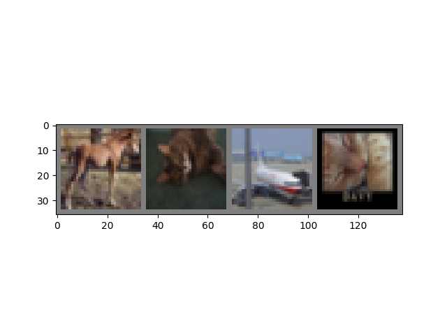
truck plane plane horse
2. 定义卷积神经网络#
从“神经网络”部分复制神经网络,并修改它以接受 3 通道图像(而不是之前定义的 1 通道图像)。
import torch.nn as nn
import torch.nn.functional as F


class Net(nn.Module):
    def __init__(self):
        super().__init__()
        self.conv1 = nn.Conv2d(3, 6, 5)
        self.pool = nn.MaxPool2d(2, 2)
        self.conv2 = nn.Conv2d(6, 16, 5)
        self.fc1 = nn.Linear(16 * 5 * 5, 120)
        self.fc2 = nn.Linear(120, 84)
        self.fc3 = nn.Linear(84, 10)

    def forward(self, x):
        x = self.pool(F.relu(self.conv1(x)))
        x = self.pool(F.relu(self.conv2(x)))
        x = torch.flatten(x, 1) # flatten all dimensions except batch
        x = F.relu(self.fc1(x))
        x = F.relu(self.fc2(x))
        x = self.fc3(x)
        return x


net = Net()
3. 定义损失函数和优化器#
让我们使用分类交叉熵损失和带动量的 SGD。
import torch.optim as optim

criterion = nn.CrossEntropyLoss()
optimizer = optim.SGD(net.parameters(), lr=0.001, momentum=0.9)
4. 训练网络#
这时事情开始变得有趣起来。我们只需遍历数据迭代器,将输入馈送到网络并进行优化。
for epoch in range(2):  # loop over the dataset multiple times

    running_loss = 0.0
    for i, data in enumerate(trainloader, 0):
        # get the inputs; data is a list of [inputs, labels]
        inputs, labels = data

        # zero the parameter gradients
        optimizer.zero_grad()

        # forward + backward + optimize
        outputs = net(inputs)
        loss = criterion(outputs, labels)
        loss.backward()
        optimizer.step()

        # print statistics
        running_loss += loss.item()
        if i % 2000 == 1999:    # print every 2000 mini-batches
            print(f'[{epoch + 1}, {i + 1:5d}] loss: {running_loss / 2000:.3f}')
            running_loss = 0.0

print('Finished Training')
[1,  2000] loss: 2.171
[1,  4000] loss: 1.850
[1,  6000] loss: 1.662
[1,  8000] loss: 1.594
[1, 10000] loss: 1.540
[1, 12000] loss: 1.500
[2,  2000] loss: 1.422
[2,  4000] loss: 1.386
[2,  6000] loss: 1.369
[2,  8000] loss: 1.329
[2, 10000] loss: 1.310
[2, 12000] loss: 1.307
Finished Training
让我们快速保存训练好的模型。
PATH = './cifar_net.pth'
torch.save(net.state_dict(), PATH)
有关保存 PyTorch 模型的更多详细信息,请参见 此处。
5. 在测试数据上测试网络#
我们对训练数据集进行了 2 个周期的训练。但我们需要检查网络是否真的学到了一些东西。
我们将通过预测神经网络输出的类别标签,并将其与真实标签进行比较来检查这一点。如果预测正确,我们就将该样本添加到正确预测列表。
好的,第一步。让我们显示一张测试集图像,以便熟悉一下。
dataiter = iter(testloader)
images, labels = next(dataiter)

# print images
imshow(torchvision.utils.make_grid(images))
print('GroundTruth: ', ' '.join(f'{classes[labels[j]]:5s}' for j in range(4)))
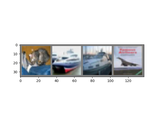
GroundTruth: cat ship ship plane
接下来,让我们重新加载保存的模型(注意:这里不一定需要保存和重新加载模型,我们只是为了演示如何操作)。
net = Net()
net.load_state_dict(torch.load(PATH, weights_only=True))
<All keys matched successfully>
好的,现在让我们看看神经网络如何看待上述示例。
输出是 10 个类别的能量值。一个类别的能量值越高,网络就越认为该图像属于该特定类别。因此,让我们获取最高能量的索引。
Predicted: cat car car plane
结果看起来相当不错。
让我们看看网络在整个数据集上的表现。
correct = 0
total = 0
# since we're not training, we don't need to calculate the gradients for our outputs
with torch.no_grad():
    for data in testloader:
        images, labels = data
        # calculate outputs by running images through the network
        outputs = net(images)
        # the class with the highest energy is what we choose as prediction
        _, predicted = torch.max(outputs, 1)
        total += labels.size(0)
        correct += (predicted == labels).sum().item()

print(f'Accuracy of the network on the 10000 test images: {100 * correct // total} %')
Accuracy of the network on the 10000 test images: 56 %
这看起来比随机猜测(随机从 10 个类别中选择一个,准确率为 10%)好多了。看来网络学到了一些东西。
嗯,哪些类别表现好,哪些类别表现不好?
# prepare to count predictions for each class
correct_pred = {classname: 0 for classname in classes}
total_pred = {classname: 0 for classname in classes}

# again no gradients needed
with torch.no_grad():
    for data in testloader:
        images, labels = data
        outputs = net(images)
        _, predictions = torch.max(outputs, 1)
        # collect the correct predictions for each class
        for label, prediction in zip(labels, predictions):
            if label == prediction:
                correct_pred[classes[label]] += 1
            total_pred[classes[label]] += 1


# print accuracy for each class
for classname, correct_count in correct_pred.items():
    accuracy = 100 * float(correct_count) / total_pred[classname]
    print(f'Accuracy for class: {classname:5s} is {accuracy:.1f} %')
Accuracy for class: plane is 64.7 %
Accuracy for class: car   is 71.7 %
Accuracy for class: bird  is 42.9 %
Accuracy for class: cat   is 40.5 %
Accuracy for class: deer  is 52.4 %
Accuracy for class: dog   is 53.2 %
Accuracy for class: frog  is 61.4 %
Accuracy for class: horse is 65.0 %
Accuracy for class: ship  is 57.4 %
Accuracy for class: truck is 55.5 %
好的,那么接下来呢?
如何在 GPU 上运行这些神经网络?
在 GPU 上训练#
就像将 Tensor 传输到 GPU 一样,您也可以将神经网络传输到 GPU。
如果我们有 CUDA 可用,让我们首先定义我们的设备为第一个可见的 CUDA 设备。
device = torch.device('cuda:0' if torch.cuda.is_available() else 'cpu')

# Assuming that we are on a CUDA machine, this should print a CUDA device:

print(device)
cuda:0
本节的其余部分假设 `device` 是一个 CUDA 设备。
然后,这些方法将递归地遍历所有模块,并将它们的参数和缓冲区转换为 CUDA Tensor。
net.to(device)
请记住,您需要在每一步将输入和目标也发送到 GPU。
为什么我没有注意到与 CPU 相比有巨大的速度提升?因为您的网络非常小。
练习: 尝试增加网络的宽度(第一个 `nn.Conv2d` 的第二个参数,以及第二个 `nn.Conv2d` 的第一个参数——它们需要相同),看看能获得多大的速度提升。
已达成目标:
高层次地理解 PyTorch 的 Tensor 库和神经网络。
训练一个小神经网络来对图像进行分类。
在多个 GPU 上训练#
如果您想使用所有 GPU 获得更大的速度提升,请参阅 可选:数据并行性。
接下来去哪里?#
del dataiter
脚本总运行时间: (1 分钟 57.226 秒)
